Semantic segmentation for autonomy future cars

I am an AI engineer in the R&D team of the “Future Vision Transport” company.

Each team member specializes in one part of the embedded computer vision system. Here are these parts of the system:

real-time image acquisition
image processing
image segmentation
decision system We focus on image segmentation.

My task in this work is to design an initial image segmentation model that will be easily integrated into the complete chain of the embedded system. We will find a model that will be further deployed as an API in order that our team can use it.

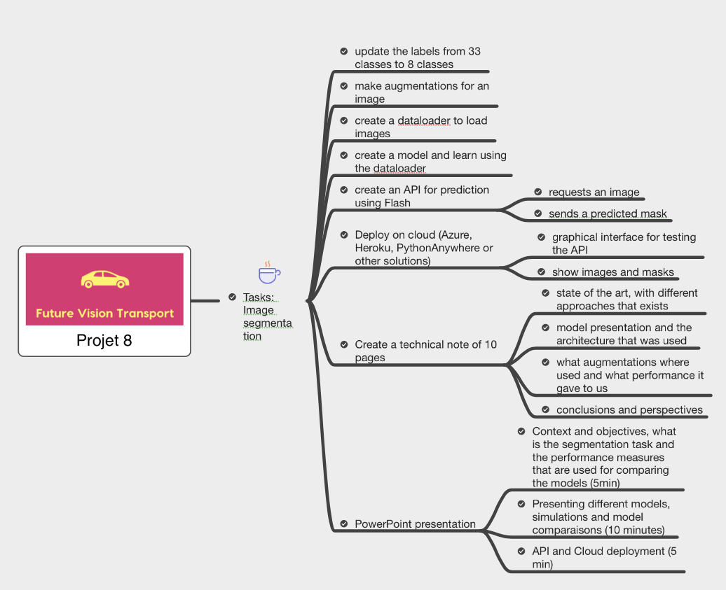
The figure bellow shows step by step what the project contains and how it will be created. First of all we will examine the Cityscapes dataset. We will see that 33 classes are in this data. We will simplify it by only supposing 8 main classes. We will use augmentation techniques and see how it can ameliorate the segmentation images modeling. We use dataloader to accelerate and permit loading the data into memory. At the end we use flask to create an API and deploy the model to one of the possible cloud services.

this is a placeholder image — Figure 1: The tasks for the Future Vision Transport project

What is semantic image segmentation?

Semantic image segmentation is a computer vision task that involves assigning a label to each pixel of an image, based on the semantic meaning of the objects or regions represented in the image. Unlike simple object detection, which involves identifying objects in an image and drawing bounding boxes around them, semantic segmentation provides a more detailed understanding of the image by labeling each pixel with a specific class.

In semantic image segmentation, the algorithm analyzes an image and assigns each pixel to one of several pre-defined categories or classes, such as “road,” “sky,” “building,” “person,” “car,” etc. This type of segmentation is often used in applications like autonomous driving, medical imaging, and robotics, where it is important to accurately identify and localize objects in an image.

Deep learning techniques, particularly convolutional neural networks (CNNs), have been very successful in solving semantic segmentation problems. By training a CNN on a large dataset of labeled images, the algorithm can learn to identify and segment objects in images with high accuracy.

Semantic image segmentation plays a crucial role in autonomous driving, as it enables the car to perceive its environment and make decisions based on the objects and features it detects. Here are some specific ways that semantic image segmentation is used in autonomous cars:

Object detection and classification: Semantic segmentation is used to detect and classify objects in the car’s environment, such as other vehicles, pedestrians, traffic signs, and lane markings.
Lane detection and tracking: Semantic segmentation is used to identify the road and the lane markings, enabling the car to stay within its lane and follow the road.
Navigation and path planning: Semantic segmentation can help the car to plan its path by identifying obstacles, intersections, and other features in the road ahead.
Pedestrian detection and avoidance: Semantic segmentation can help the car to detect and avoid pedestrians, which is crucial for ensuring the safety of pedestrians and other road users.

Overall, semantic image segmentation enables the car to perceive its environment with a high degree of accuracy, which is essential for safe and effective autonomous driving.

Importing libraries

First import the libraries. The main think to install here is the tensorflow librabry that is specific for the MACOS M1. For reference I invite you to see the youtube link. Also we install sklearn, numpy, pandas, PIL, cv2, albumations, matplotlib for this project.

Exploring the dataset

Data description

After we downloaded the Cityscapes dataset we discover it’s content and give some breaf introduction here.

The folder dataset containes the folowing :

leftImg8bit : the images of the dataset, I rename it to images/
gtFine/ : contains the images, I rename this folder into masks/
test/, train/ and val/ : contains the the three splits of the dataset
berlin/, frankfurt/, munich/, … : contains the images that corresponds to different cities
*_gtFine_color.png : contains the labels colors
*_gtFine_instanceIds.png : contains the instance ids
*_gtFine_labalIds.png : contains the label ids
*_gtFine_polygons.json : contains the polygon shapes

We are not going to use the polygon shapes, but we will use the instance ids to build the ground truth images.

The dataset contains :

2975 train images
500 validation images
1525 test images

According to the Cityscapes dataset documentation, the images are of size 2048x1024 and are in RGB format.

We will not use the object labels (32 labels), but the 8 label categories : “void”, “flat”, “construction”, “object”, “nature”, “sky”, “human” and “vehicle”.

Firstly, we load the images and masks as train, validation, and test datasets, sorted in a way that aligns them. Let us now write the files that will be in future used for our data generation:

train_input_img_paths
train_label_ids_img_paths
val_input_img_paths
val_label_ids_img_paths
test_input_img_paths
test_label_ids_img_paths

print('We have {0} train images'.format(len(train_input_img_paths)))
print('We have {0} validation images'.format(len(val_input_img_paths)))
print('We have {0} test images'.format(len(test_input_img_paths)))

We have 2974 train images
We have 500 validation images
We have 1525 test images

In the next step, we will take a random image and attempt to identify every file that pertains to that specific ID of the image.

rand_idx = np.random.randint(0, len(val_input_img_paths))
image_id = (
    str(val_input_img_paths[rand_idx])
    .split("/")[-1]
    .replace("_leftImg8bit.png", "")
)
img = np.array(Image.open(val_input_img_paths[rand_idx]))
ids_img = np.array(np.array(Image.open(val_label_ids_img_paths[rand_idx])))
img_size = img.shape
color_img = np.array(np.array(Image.open(val_label_colors_img_paths[rand_idx])))
ids_img_size = ids_img.shape
color_img_size = color_img.shape

print('The size image is: {0}'.format(img_size))
print('The size ids image is: {0}'.format(ids_img_size))
print('The size color image is: {0}'.format(color_img_size))

The size image is: (1024, 2048, 3)
The size ids image is: (1024, 2048)
The size color image is: (1024, 2048, 4)

W e observe the following information about theese images:

each image has the size of (1024, 2048) with dimension 3 that is the RGB.
the label_ids images sizes are (1024, 2048) that tells us the label associated to that pixel
color image has the size of (1024, 2048) with dimension 4. The first 3 dimensions is the RGB and the fourth layer is the alpha chanel which is added to allow the transparency of the image (it does not change the color of the pixel). Also, we note that this is equal to 255 for all the times, there is why we can delete it.

Also we say there are 1024 * 2048 = 2097152 pixels in the image.

Let us see, for exaple, the color of the first pixel in the image

img[0,0,:]

array([34, 45, 62], dtype=uint8)

Let us see the ids of the first pixel in the labelIds image.

ids_img[0,0]

This correspons to 3, that meens that the first pixel is attributed to the void cathegory. And how about the unique values in the ids image.

np.unique(ids_img)

array([ 1,  2,  3,  4,  5,  7,  8, 11, 12, 17, 19, 20, 21, 22, 23, 24, 25,
       26, 33], dtype=uint8)

len(np.unique(ids_img))

There are 19 different labels for this particular image, however the maximum number of classes is 33.

Colors in the image

Examining the colors of the particular image and counting each of theese colors we obtain the following:

colours, counts = np.unique(color_img.reshape(-1,3), axis=0, return_counts=1)
for j in range(len(colours)):
    print('{0}/{1}:{2}'.format(j, colours[j], counts[j]))

0/[0 0 0]:276171
1/[  0   0 142]:19697
2/[70 70 70]:240320
3/[ 70 130 180]:95763
4/[102 102 156]:7754
5/[107 142  35]:428094
6/[111  74   0]:1804
7/[119  11  32]:31545
8/[128  64 128]:852620
9/[152 251 152]:4334
10/[153 153 153]:50127
11/[220  20  60]:4529
12/[220 220   0]:3501
13/[244  35 232]:63408
14/[250 170  30]:3663
15/[255   0   0]:13822

Image anotation

Let us now discover how the images had been annotated. We define a function that counts the label anotation for a specific image.

def count_label_anotation(ann_img):
    colours, counts = np.unique(ann_img, return_counts=1)
    for j in range(len(colours)):
        print('{0}/{1}:{2}'.format(j, colours[j], counts[j]))

We observe the 19 classes as we saw for this image. In this project we are asked to transform our data to obtain 8 class annotation. This is discussed in the next section.

count_label_anotation(ids_img)

0/1:121096
1/2:74098
2/3:31634
3/4:49343
4/5:1804
5/7:852620
6/8:63408
7/11:240320
8/12:7754
9/17:50127
10/19:3663
11/20:3501
12/21:428094
13/22:4334
14/23:95763
15/24:4529
16/25:13822
17/26:19697
18/33:31545

Transform 8 classes annotation

cats_replace = {0: [0, 1, 2, 3, 4, 5, 6], # void
[7, 8, 9, 10], # flat
[11, 12, 13, 14, 15, 16], # construction
[17, 18, 19, 20], # object
[21, 22], # nature
[23], # sky
[24, 25], # human
[26, 27, 28, 29, 30, 31, 32, 33, -1] # vehicle
 }

mask_labelids = pd.DataFrame(ids_img)
for new_value, old_value in cats_replace.items():
    mask_labelids = mask_labelids.replace(old_value, new_value);
mask_labelids = mask_labelids.to_numpy()

count_label_anotation(mask_labelids)

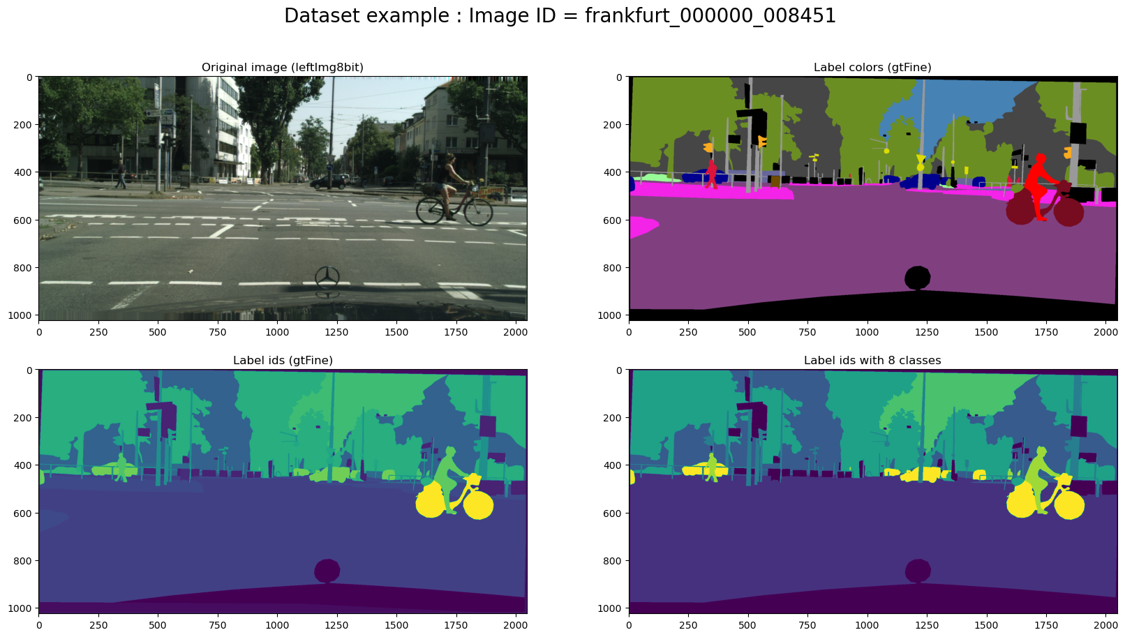
Observe that the picture shows all 8 required classes after replacing the old values classes. Let us examine the original image in conjunction with its annotation.

# plot images
fig, ax = plt.subplots(
    nrows=2,
    ncols=2,
    figsize=(20, 10),
)
fig.suptitle(f"Dataset example : Image ID = {image_id}", fontsize=20)

ax[0, 0].title.set_text("Original image (leftImg8bit)")
ax[0, 0].imshow(img)

ax[0, 1].title.set_text("Label colors (gtFine)")
ax[0, 1].imshow(color_img)

ax[1, 0].title.set_text("Label ids (gtFine)")
ax[1, 0].imshow(np.array(ids_img))

ax[1, 1].title.set_text("Label ids with 8 classes")
ax[1, 1].imshow(np.array(mask_labelids))

plt.show()

Resizing Image and the Mask

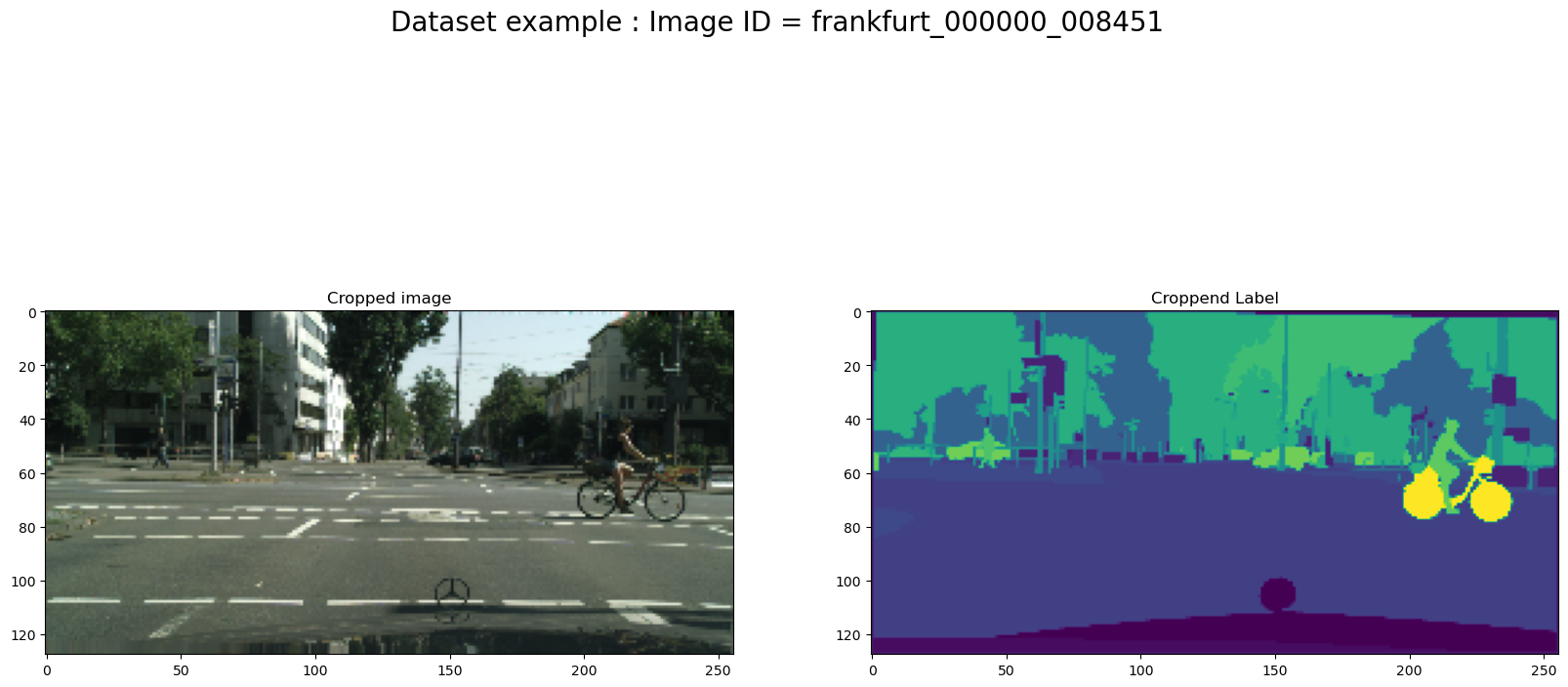
We also demonstrate how to resize the image using the CV2 library.

import cv2
X = np.array(cv2.resize(cv2.cvtColor(cv2.imread(str(val_input_img_paths[rand_idx])), cv2.COLOR_BGR2RGB), (256, 128)))
y = np.array(cv2.resize(cv2.imread(str(val_label_ids_img_paths[rand_idx]),0), (256, 128)))

# plot images
fig, ax = plt.subplots(
    nrows=1,
    ncols=2,
    figsize=(20, 10),
)
fig.suptitle(f"Dataset example : Image ID = {image_id}", fontsize=20)

ax[0].title.set_text("Cropped image")
ax[0].imshow(X)

ax[1].title.set_text("Croppend Label")
ax[1].imshow(y)

Augmentation images

Data augmentation is a powerful technique to increase the amount of your data and prevent model overfitting. If you not familiar with such trick read some of these articles:

The Effectiveness of Data Augmentation in Image Classification using Deep Learning

Data Augmentation | How to use Deep Learning when you have Limited Data Data Augmentation Experimentation Since our dataset is very small we will apply a large number of different augmentations:

horizontal flip
affine transforms
perspective transforms
brightness/contrast/colors manipulations
image bluring and sharpening
gaussian noise
random crops

All this transforms can be easily applied with Albumentations - fast augmentation library. For detailed explanation of image transformations you can look at kaggle salt segmentation exmaple provided by Albumentations authors.

Let us now see an exemple of how we can augment the images. We will take the original image and the label ids with 8 annotated classes and we will use the albumentations class to augment the images.

transform = aug.Compose(
    [
        aug.OneOf(  # Color augmentations
            [
                aug.RandomBrightnessContrast(),
                aug.RandomGamma(),
                aug.RandomToneCurve(),
            ]
        ),
        aug.OneOf(  # Camera augmentations
            [
                aug.MotionBlur(),
                aug.GaussNoise(),
            ]
        ),
        aug.OneOf(  # Geometric augmentations
            [
                aug.HorizontalFlip(),
                aug.RandomCrop(
                    width=int(img_size[1] / random.uniform(1.0, 2.0)),
                    height=int(img_size[0] / random.uniform(1.0, 2.0)),
                ),
                aug.SafeRotate(
                    limit=15,
                ),
            ]
        ),
    ]
)

augmented = transform(
    image=img,
    mask=mask_labelids,
)

# plot images
fig, ax = plt.subplots(
    nrows=2,
    ncols=2,
    figsize=(20, 10),
)
fig.suptitle(f"Dataset example : Image ID = {image_id}", fontsize=20)

ax[0,0].title.set_text("Original image (leftImg8bit)")
ax[0,0].imshow(img)

ax[0,1].title.set_text("Original Label ids with 8 classes")
ax[0,1].imshow(np.array(mask_labelids))

ax[1,0].title.set_text("Augmented image")
ax[1,0].imshow(np.array(augmented["image"]))

ax[1,1].title.set_text("Augmented mask")
ax[1,1].imshow(np.array(augmented["mask"]))

plt.show()

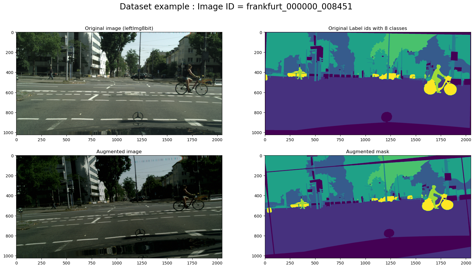
In figure 4, I demonstrate how data can be augmented on images. To improve the final results, this step must be reviewed during the training model step. You can see my final augmentation code in my github account. I will share the link to the project at the end of this article.

Dataset and DataLoader

Because of the data that is imposible to load in memory we will take advantage of the data loader that is an essential component in machine learning pipelines that deal with large datasets.

To give some motivation and reasons of why we use DataLoader:

Memory management: DataLoader allows us to load only a subset of the data into memory at a time, which is important for handling large datasets that may not fit in memory. By loading data in batches, we can reduce memory usage and avoid memory errors.
Efficiency: DataLoader can help to improve the efficiency of the training process by pre-fetching data in the background while the model is processing the current batch of data. This reduces the idle time that the model would otherwise spend waiting for data to load.
Data augmentation: DataLoader can be used to apply data augmentation techniques such as flipping, rotating, and cropping to the data before it is fed into the model. This helps to increase the size and diversity of the dataset, which can improve the accuracy of the model.
Parallel processing: DataLoader can be used to load data in parallel from multiple sources, which can improve the speed of the training process on multi-core systems. O verall, DataLoader provides a convenient and efficient way to handle large datasets and improve the performance of machine learning models.

I create the dataset class and the dataloader class in my_classes.py, that can be viewed in the github repository of this project.

Let us make a test of loading the data with DataLoader and Dataset class. We will also use the augmentation technique inside the Dataset class.

# Lets look at augmented data we have
x_train_dir = 'train_images.txt'
y_train_dir = 'train_mask.txt'
image_id = 10
dataset = mc.Dataset(x_train_dir, y_train_dir)
dataset_aug = mc.Dataset(x_train_dir, y_train_dir, augmentation=get_training_augmentation())
image, mask = dataset[image_id] # get some sample
image_aug, mask_aug = dataset_aug[image_id] # get some sample

# plot images
fig, ax = plt.subplots(
    nrows=1,
    ncols=2,
    figsize=(20, 10),
)
fig.suptitle(f"Dataset example : Image ID = {image_id}", fontsize=20)

ax[0].title.set_text("Original image (leftImg8bit)")
ax[0].imshow(image)

ax[1].title.set_text("Original Label ids with 8 classes")
ax[1].imshow(np.argmax(mask, 2))


plt.show()

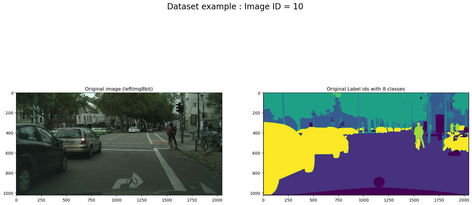
Figure 5 demonstrates the original image and the corresponding mask. We used the DataLoader Class to load the dataset in memory.

fig, ax = plt.subplots(
    nrows=1,
    ncols=2,
    figsize=(20, 10),
)
fig.suptitle(f"Dataset augmented example : Image ID = {image_id}", fontsize=20)

ax[0].title.set_text("Augmented Image (leftImg8bit)")
ax[0].imshow(image_aug)

ax[1].title.set_text("Augmented mask with 8 classes")
ax[1].imshow(np.argmax(mask_aug, 2))

plt.show()

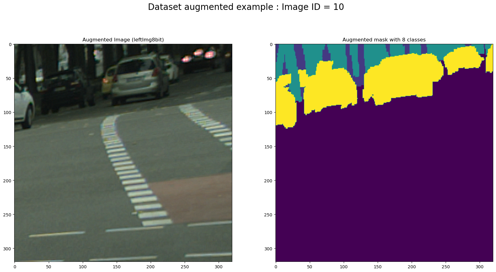
Figure 6 shows the same as for Figure 5, but with using the augmentation of the data in the DataLoader class.

It seems that everithing is working as it was expected. I am moving to the next step that is the modeling step where we create the segmentation models.

Modeling: Sematic segmentation

Semantic segmentation is typically performed using a type of neural network called a Fully Convolutional Network (FCN). FCNs are designed to take an input image and produce a dense output, where each pixel in the output image is assigned a label.

The output of semantic segmentation can be used in a wide range of applications, such as self-driving cars, robotics, and image retrieval. It can also be useful for image editing and image understanding tasks.

It is a supervised learning task, where the model is trained on a labeled dataset, where each pixel in the image is assigned a label. The model then uses this training data to learn the relationship between the pixels and the semantic labels, and can then generalize this knowledge to new images.

There are many semantic segmentation algorithms such as U-net, Mask R-CNN, Feature Pyramid Network (FPN), etc. This work is mainly focused on U-net. In the state of the art, we find the UNet is a deep learning architecture with a high performance for image segmentation.

What is UNet?

UNet is a type of neural network architecture that is used for image segmentation tasks, it was first introduced in 2015 by Olaf Ronneberger, Philipp Fischer, and Thomas Brox.

The architecture of UNet is composed of two parts: an encoder and a decoder. The encoder is a traditional convolutional neural network that is used to extract features from the input image. The decoder is then used to generate the segmentation mask.

1) A contracting path that is similar to the encoder. This caputres the context via a compact feature map. 2) A symetric expanding path that is the decoder. This allows a precise localisation. This step is done to make boundary information (spacial information).

The encoder and decoder are then connected by a set of “skip” connections, which allow the decoder to access the feature maps generated by the encoder. This allows the decoder to combine the high-level, semantic features of the encoder with the fine-grained details of the input image.

Here is the architecture of U-Net based on the original paper:

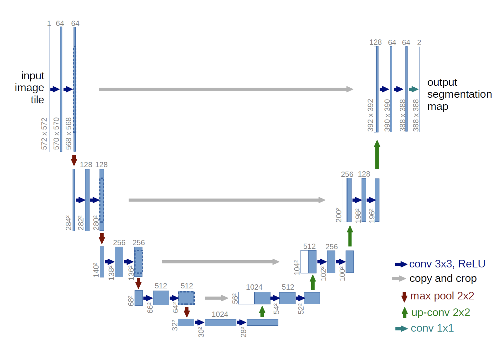
UNet has been widely used in various fields such as medical imaging, self-driving cars, and many other computer vision tasks.

UNet in practice

UNet Model (without augmentation)

import segmentation_models as sm
print(f"segmentation_models Version: {sm.__version__}")

Segmentation Models: using `keras` framework.
segmentation_models Version: 1.0.1

As you have noticed I will use a package that is the Segmentation models (https://github.com/qubvel/segmentation_models) python library available online.

@misc{Yakubovskiy:2019,
  Author = {Pavel Iakubovskii},
  Title = {Segmentation Models},
  Year = {2019},
  Publisher = {GitHub},
  Journal = {GitHub repository},
  Howpublished = {\url{https://github.com/qubvel/segmentation_models}}
}

The main features of this library are:

High level API (just two lines of code to create model for segmentation)
4 models architectures for binary and multi-class image segmentation (including legendary Unet)
25 available backbones for each architecture
All backbones have pre-trained weights for faster and better convergence
Helpful segmentation losses (Jaccard, Dice, Focal) and metrics (IoU, F-score)

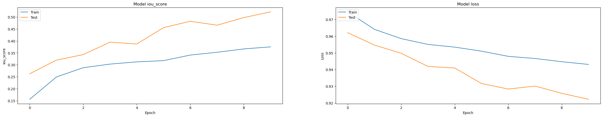
Now, we give the batch size = 8, learning rate = 0.0001 and we learn our model for 10 epochs. We learn an Unet for our 8 classes labeled dataset using the Adam optimizer. The dice loss is used here to optimize the model.

# train model
history_without_aug = model.fit_generator(
    train_dataloader, 
    steps_per_epoch=len(train_dataloader), 
    epochs=EPOCHS, 
    callbacks=callbacks, 
    validation_data=valid_dataloader, 
    validation_steps=len(valid_dataloader),
)

The following code is used to save and load the model:

import pickle
pickle.dump(history_without_aug, open("history_without_aug.pkl", "wb"))
model.load_weights('best_model_without_aug.h5') 

Let us evaluate our model by regarding the iou score and the f1 score.

scores = model.evaluate_generator(test_dataloader)

print("Loss: {:.5}".format(scores[0]))
for metric, value in zip(metrics, scores[1:]):
    print("mean {}: {:.5}".format(metric.__name__, value))

Loss: 0.92215
mean iou_score: 0.52147
mean f1-score: 0.62958

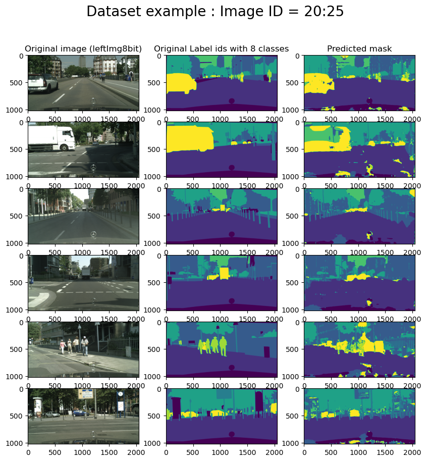
Also, let us predict the segmentation on 6 images using the obtained model.

image_id = 20
image_id_end = 26

# plot images
fig, ax = plt.subplots(
    nrows=image_id_end - image_id,
    ncols=3,
    figsize=(10, 10),
)
fig.suptitle("Dataset example : Image ID = {0}:{1}".format(image_id,image_id_end-1), fontsize=20)


for row, i in enumerate(range(image_id, image_id_end)):
    image, mask = test_dataset[i]
    image_origin, mask_origin = test_dataset_origin[i]

    image = np.expand_dims(image, axis=0)
    pr_mask = model.predict(image)
    
    if row==0:
        ax[row, 0].title.set_text("Original image (leftImg8bit)")
        ax[row, 1].title.set_text("Original Label ids with 8 classes")
        ax[row, 2].title.set_text("Predicted mask")
        
    ax[row, 0].imshow(image_origin.squeeze())
    ax[row, 1].imshow(np.argmax(mask_origin, 2))
    ax[row, 2].imshow(np.argmax(pr_mask.squeeze(), 2))
    
plt.show()

1/1 [==============================] - 1s 931ms/step
1/1 [==============================] - 1s 506ms/step
1/1 [==============================] - 0s 443ms/step
1/1 [==============================] - 0s 444ms/step
1/1 [==============================] - 0s 454ms/step
1/1 [==============================] - 0s 448ms/step

UNet Model (with augmentation)

Now, we train the same UNet model but with making augmentation on the dataset. Let us see how the model can be improved.

# train model
history = model.fit_generator(
    train_dataloader, 
    steps_per_epoch=len(train_dataloader), 
    epochs=EPOCHS, 
    callbacks=callbacks, 
    validation_data=valid_dataloader, 
    validation_steps=len(valid_dataloader),
)

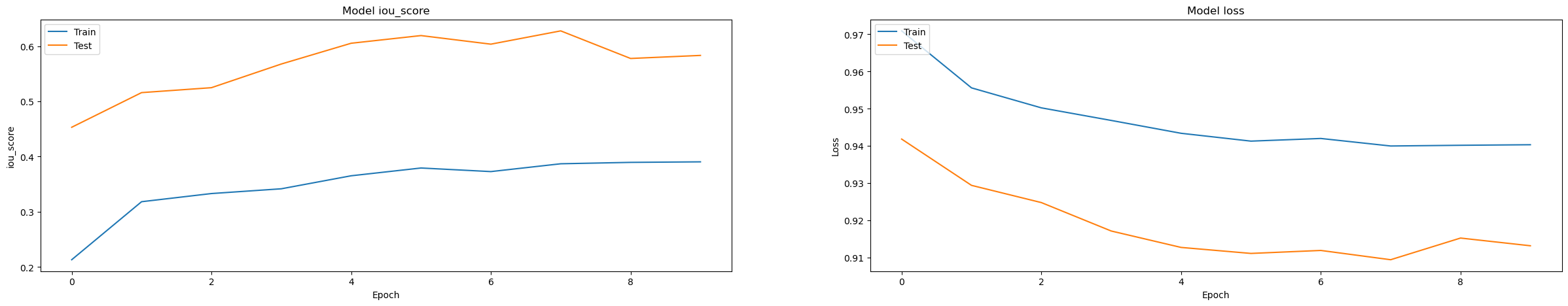
We already have seen how we save the model. This will be used in future when we deploy it on the cloud. Here are the results obtained for the approach with using the augmented data.

Loss: 0.90948
mean iou_score: 0.62761
mean f1-score: 0.73222

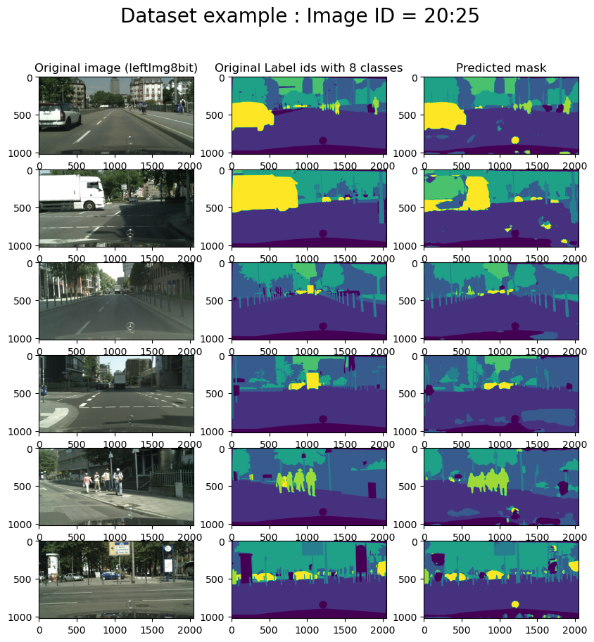
We predict the masks for the same images as in the previous example. We see the improvements on the predicted mask.

Results

We train the U-Net models using the segmentation models python package with/without Data augmentations using the data loader that we created. Furthermore, we use a batch size of 8 and reduce the images to 320 × 320 pixels. I run the learning for 10 epochs (this is because the learning is done on a personal computer, and it demands a lot of time and resources). Furthermore, I also used a pre-trained network weight that is efficientnetb3. This backbone permits us to converge faster. We compare the results of having the augmentation on images and using the images without any augmentations on learning.

One can see better performance in learning the U-Net on augmented images and using a pre-trained network. Comparing the IOU, we observe that the score obtained without augmenting the data is 0.52 and the score by augmenting the data is for 0.62.

Of course, this work is done for a presentation purpose and can not be used directly on an autonomous car system. Therefore, I present some conclusions and perspectives for this work.

Deployment

For deployment of our application we used the doker. First we created our docker on the local machine, then we pushed it to the Container Registry of Google cloud and the we used Google Run to run our API.

# start by pulling the python image
FROM python:3.9-slim-buster

# update the pip
RUN pip install --upgrade pip

# update setuptools and wheel
RUN pip install --upgrade setuptools wheel

# copy the requirements file into the image
COPY ./requirements.txt /app/requirements.txt

# switch working directory
WORKDIR /app

# install the dependencies and packages in the requirements file
RUN pip install -r requirements.txt

# copy every content from the local file to the image
COPY . /app

# configure the container to run in an executed manner
ENTRYPOINT [ "python" ]

CMD ["main.py" ]

We used streamlit to develop a web application that we deployed also on google cloud.

Here are some example of the deployed application:

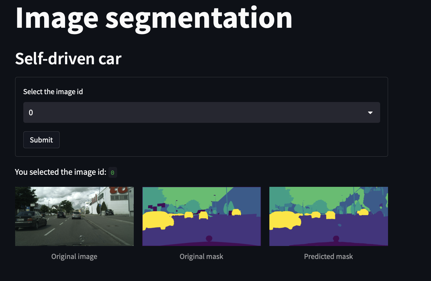
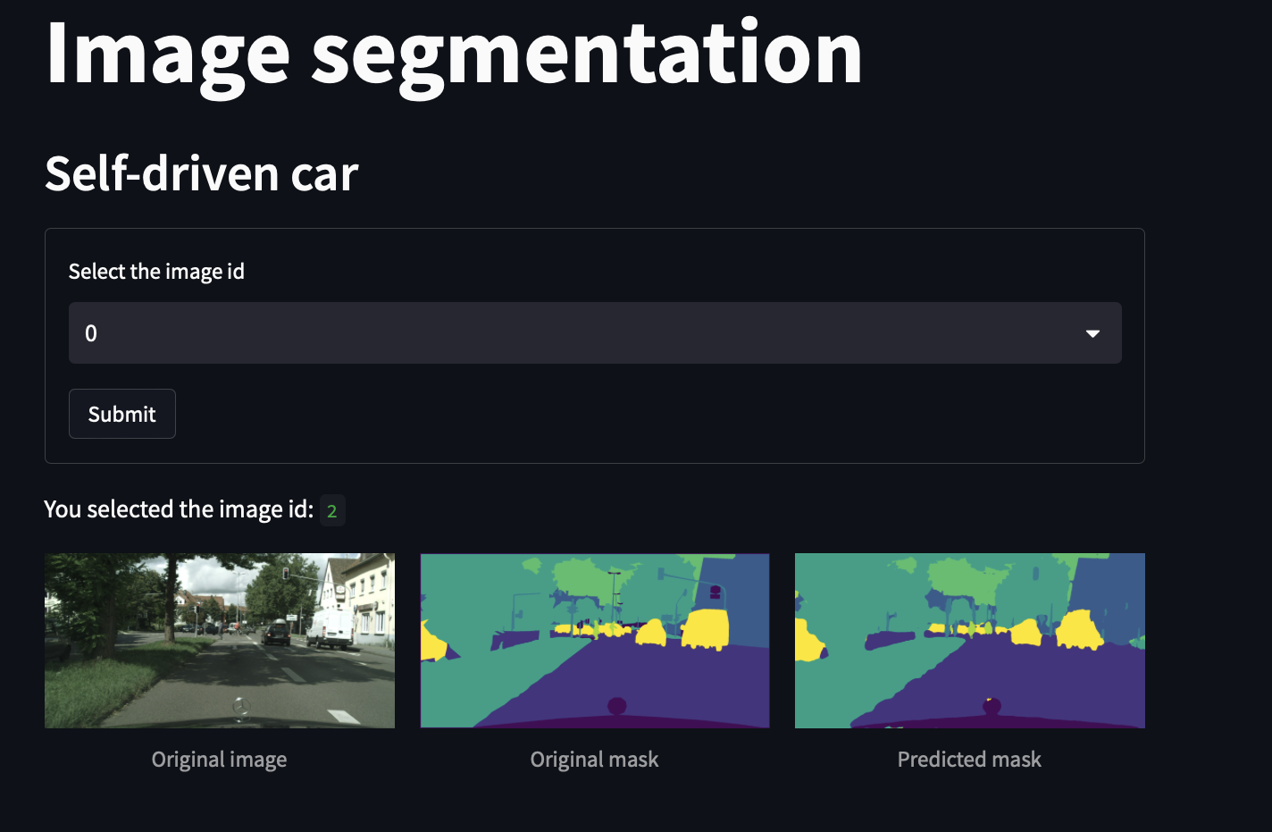
Conclusions and perspectives

In this work, we saw semantic segmentation and how we apply it to the self-driving car problem. We designed an initial image segmentation model that will be easily integrated into the complete chain of the embedded system. A segmentation model had been computed. We saw how we can train a segmentation model, particularly U-Net, with and without augmentation images. Interesting and presentable results were found, however, some improvements could be done in future work.

In order to improve the model, different things can be taken into consideration:

a larger dataset, taking more images to learn. Even if the dataset is large, a bigger and more vast dataset can always improve a model.
We reduced the images to 320 x 320. Taking a bigger image can ameliorate our model.
Make some different augmentation of the data.
Giving a higher number of batches.
Optimize the hyperparameters, like the learning rate.
Learning with a higher number of epochs.
Trying other models than UNet that can be more performant.

All of these tasks need more resources: a highly performant computer and more time.

Twitter Facebook LinkedIn

Role

Responsibilities