
Prepare data for a public health agency
This project is focused on data gathered from the public health agency of France. The data information and description can be found on the OpenFoodData website: OpenFood.
The main tasks of the project were to:
1) Process the dataset to identify relevant variables for further processing. Automate these processes to avoid repeating these operations. The program should work if the database is slightly modified (e.g. adding entries).
2) Throughout the analysis, produce visualizations to better understand the data. Perform a univariate/multivariate analysis for each variable of interest to summarise its behavior.
3) Confirm or refute hypotheses using descriptive and explanatory multivariate analysis. Perform appropriate statistical tests (one descriptive, one explanatory) to check the significance of the results.
In the figure below, I describe what is realized in this work.
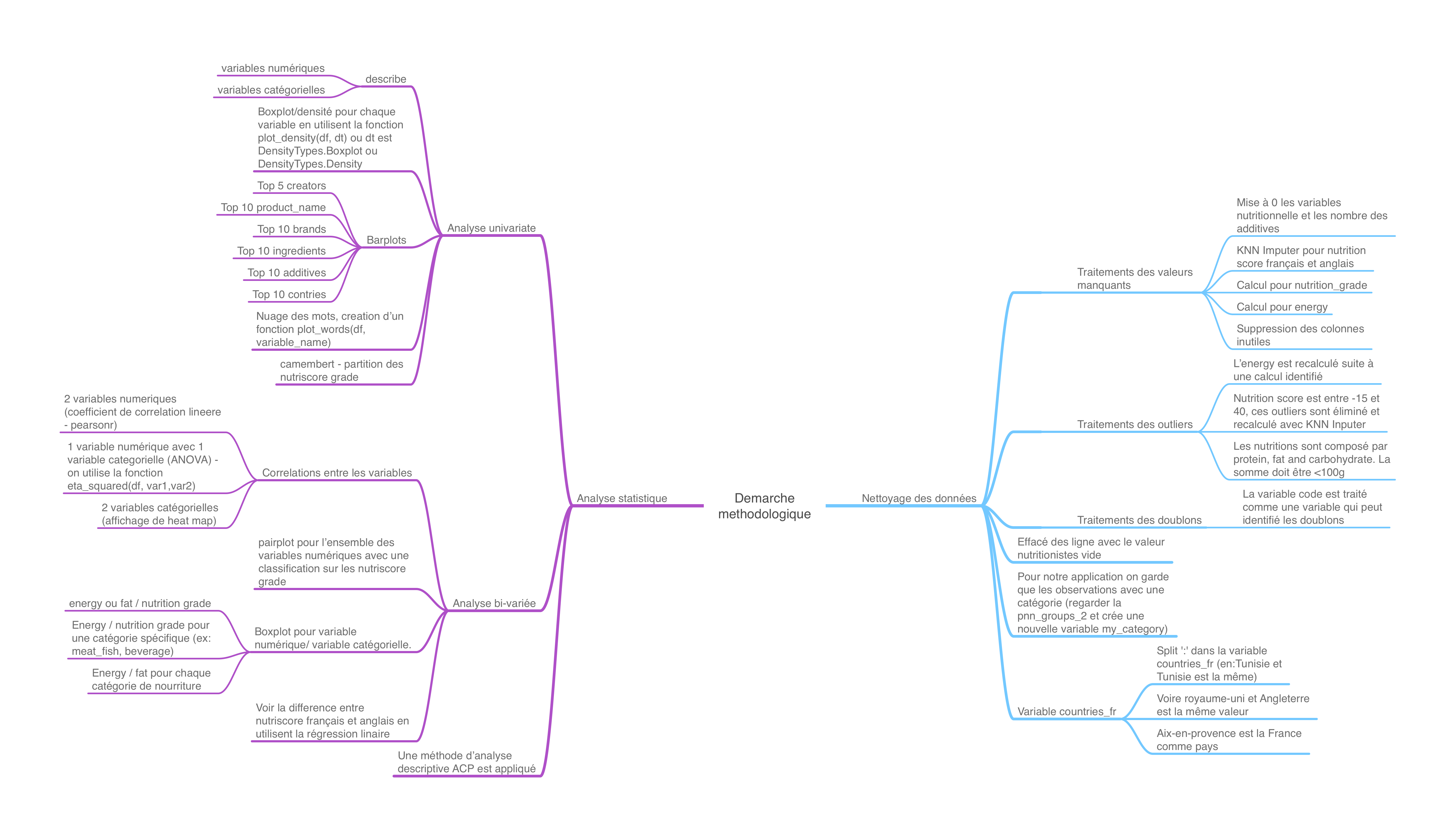
Nevertheless, the first thing to do was to select a problem and describe it.
Problem description:Permalink
We all have our own preferences when it comes to food. There are some who are interested in meat or fish, others who are interested in cheese, and still others who are interested in beverages. In addition, we wish to maintain our health by consuming the best foods.
It is, however, difficult to make an informed decision due to the wide variety of these foods accompanied by a myriad of nutrition facts.
Below are some nutrition facts and information to assist you in making the right food choices:
Our bodies store excess calories as body fat when we consume more calories than we burn. We may gain weight if this trend continues.
It is essential for your body to have fats in order to provide energy to your cells and support their function. By keeping your body warm, they also protect your organs. It is important to note that fats help the body absorb some nutrients as well as produce important hormones.
-
Carbohydrates are your body’s main source of energy: They help fuel your brain, kidneys, heart muscles, and central nervous system. For instance, fiber is a carbohydrate that aids digestion, helps you feel full, and keeps blood cholesterol levels in check.
-
Sugars higher blood pressure, inflammation, weight gain, diabetes, and fatty liver disease — are all linked to an increased risk of heart attack and stroke.
-
The human body requires a small amount of sodium to conduct nerve impulses, contract and relax muscles, and maintain the proper balance of water and minerals. It is estimated that we need about 500 mg of sodium daily for these vital functions.
We have to take control of the foods we are consuming. An active lifestyle can require more energy. Others need to eat less fatty foods and live a less active life, like having an inactive job. It is possible for others with certain desires to be restricted from eating foods containing some nutrients, such as sugars, salts, or additives.
In my data analysis project, I propose to analyze the nutrition of food facts. I also propose an application to help the user understand the food nutrition facts, and make a decision on the desired food.
Importing librariesPermalink
First import libraries.
import pandas as pd
import numpy as np
import matplotlib.pyplot as plt
import seaborn as sns

import scipy.stats as st

from sklearn import decomposition
from sklearn import preprocessing
from functions import *
from utils import *

from IPython.core.interactiveshell import InteractiveShell

InteractiveShell.ast_node_interactivity = "all"
Loading datasetPermalink
df = pd.read_csv('data/fr_openfoodfacts_products.csv', sep = '\t', encoding='utf-8', decimal='.', low_memory=False)
#df = data.copy()
df.head(5)
| code | url | creator | created_t | created_datetime | last_modified_t | last_modified_datetime | product_name | generic_name | quantity | ... | ph_100g | fruits-vegetables-nuts_100g | collagen-meat-protein-ratio_100g | cocoa_100g | chlorophyl_100g | carbon-footprint_100g | nutrition-score-fr_100g | nutrition-score-uk_100g | glycemic-index_100g | water-hardness_100g | |
|---|---|---|---|---|---|---|---|---|---|---|---|---|---|---|---|---|---|---|---|---|---|
| 0 | 0000000003087 | http://world-fr.openfoodfacts.org/produit/0000... | openfoodfacts-contributors | 1474103866 | 2016-09-17T09:17:46Z | 1474103893 | 2016-09-17T09:18:13Z | Farine de blé noir | NaN | 1kg | ... | NaN | NaN | NaN | NaN | NaN | NaN | NaN | NaN | NaN | NaN |
| 1 | 0000000004530 | http://world-fr.openfoodfacts.org/produit/0000... | usda-ndb-import | 1489069957 | 2017-03-09T14:32:37Z | 1489069957 | 2017-03-09T14:32:37Z | Banana Chips Sweetened (Whole) | NaN | NaN | ... | NaN | NaN | NaN | NaN | NaN | NaN | 14.0 | 14.0 | NaN | NaN |
| 2 | 0000000004559 | http://world-fr.openfoodfacts.org/produit/0000... | usda-ndb-import | 1489069957 | 2017-03-09T14:32:37Z | 1489069957 | 2017-03-09T14:32:37Z | Peanuts | NaN | NaN | ... | NaN | NaN | NaN | NaN | NaN | NaN | 0.0 | 0.0 | NaN | NaN |
| 3 | 0000000016087 | http://world-fr.openfoodfacts.org/produit/0000... | usda-ndb-import | 1489055731 | 2017-03-09T10:35:31Z | 1489055731 | 2017-03-09T10:35:31Z | Organic Salted Nut Mix | NaN | NaN | ... | NaN | NaN | NaN | NaN | NaN | NaN | 12.0 | 12.0 | NaN | NaN |
| 4 | 0000000016094 | http://world-fr.openfoodfacts.org/produit/0000... | usda-ndb-import | 1489055653 | 2017-03-09T10:34:13Z | 1489055653 | 2017-03-09T10:34:13Z | Organic Polenta | NaN | NaN | ... | NaN | NaN | NaN | NaN | NaN | NaN | NaN | NaN | NaN | NaN |
5 rows × 162 columns
EDAPermalink
# quantité des données
print('Les quantité des données')
df.shape

# regarder les type des variable
print('Les type observé pour chaque variable')
df.dtypes

print('Conté les type des variables')
df.dtypes.value_counts()
Les quantité des données

(320772, 162)

Les type observé pour chaque variable

code                        object
url                         object
creator                     object
created_t                   object
created_datetime            object
                            ...
carbon-footprint_100g      float64
nutrition-score-fr_100g    float64
nutrition-score-uk_100g    float64
glycemic-index_100g        float64
water-hardness_100g        float64
Length: 162, dtype: object

Conté les type des variables

float64    106
object      56
dtype: int64
We observe:
- Observations and variables: 320772, 162
- Types des variables: qualitative: 56 quantitative: 106
Filtering data. Cleaning data.Permalink
# verifié les valeurs manquants en affichant le pourcentage
dd = df.isna().mean().sort_values(ascending=True)*100

fig = plt.figure(figsize=(15, 10));
axes = sns.barplot(x=dd.values, y=dd.index, data=dd);
axes.set_xticks([]);
axes.set_yticks([0, 20, 40, 60, 80, 100]);
plt.title('NaN Values on entire dataset',fontsize=25);
plt.xlabel('Variables',fontsize=15);
plt.ylabel('% of NaN values',fontsize=15);
del dd;
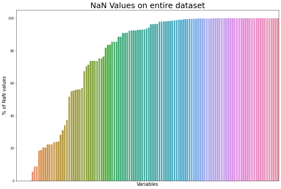
We observe:
- 162 variables with lots of NaNs! We should try to find an application and select the necessary variables!
First, for more clarity, we can see the variables that are less than 40% of NaNs.
var_verify = (df.isna().mean() < 0.4)
columns40 = list(df.columns[var_verify])
The purpose of my data analysis project is to analyze the nutritional information provided by food facts. Additionally, I propose a software application that helps users understand food nutrition facts and make food choices.
Despite the fact that there are other important variables in the dataset, these are the most important features for our first data analysis. For the purpose of identifying the product, we utilize the following features:
-
Product information:
codecreatorbrandsproduct_namecountries_fringredients_textserving_sizeadditives_ningredients_from_palm_oil_ningredients_that_may_be_from_palm_oil_nadditives_tagspnns_groups_2
- The nutritions value used to compute the nutri score
energy_100gfat_100gsaturated-fat_100gcarbohydrates_100gsugars_100gfiber_100gproteins_100gsalt_100gsodium_100gfruits-vegetables-nuts_100g
- The nutri score
nutrition_grade_frnutrition-score-fr_100gnutrition-score-uk_100g
selected_columns = []

if 'fruits-vegetables-nuts_100g' not in columns40:
    columns40.append('fruits-vegetables-nuts_100g') # needed to compute the nutri-score

if 'pnns_groups_2' not in columns40:
    columns40.append('pnns_groups_2') # need to get categories

for c in columns40:
    if not(c.endswith('_datetime')) and not(c.endswith('_t')) and not(c.endswith('_tags')):
        selected_columns.append(c)

if 'additives_tags' not in selected_columns:
    selected_columns.append('additives_tags')

if 'additives' in selected_columns:
    selected_columns.remove('additives')

df_selected = df[selected_columns];
Now we have our data with the selected columns. The next step is to omit unnecessary columns.
Getting rid of unnecessary colonsPermalink
cols_to_delete = ['states', 'states_fr', 'countries', 'url'] # 'nutrition-score-uk_100g'

for c in cols_to_delete:
    if c in df_selected.columns:
        df_selected.drop(c, inplace=True, axis=1)
# quantité des données
print('Les quantité des données')
df_selected.shape

# regarder les type des variable
print('Les type observé pour chaque variable')
df_selected.dtypes

print('Conté les type des variables')
df_selected.dtypes.value_counts()
Les quantité des données

(320772, 25)

Les type observé pour chaque variable

code                                        object
creator                                     object
product_name                                object
brands                                      object
countries_fr                                object
ingredients_text                            object
serving_size                                object
additives_n                                float64
ingredients_from_palm_oil_n                float64
ingredients_that_may_be_from_palm_oil_n    float64
nutrition_grade_fr                          object
energy_100g                                float64
fat_100g                                   float64
saturated-fat_100g                         float64
carbohydrates_100g                         float64
sugars_100g                                float64
fiber_100g                                 float64
proteins_100g                              float64
salt_100g                                  float64
sodium_100g                                float64
nutrition-score-fr_100g                    float64
nutrition-score-uk_100g                    float64
fruits-vegetables-nuts_100g                float64
pnns_groups_2                               object
additives_tags                              object
dtype: object

Conté les type des variables


float64    15
object     10
dtype: int64
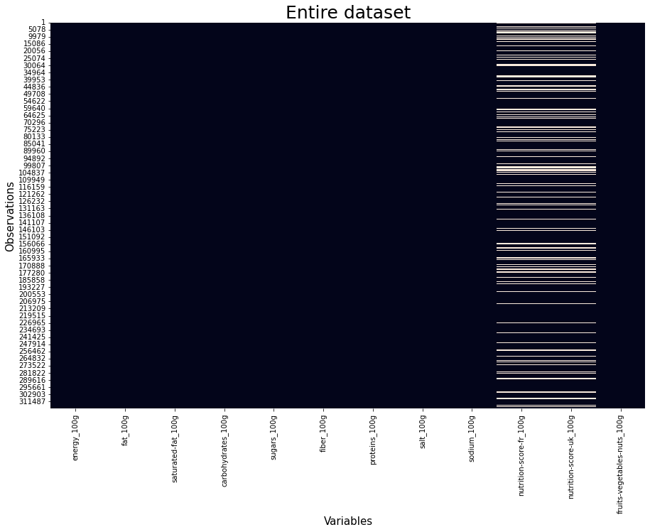
Let us now examine our data to see how many NaN values it contains.
plot_data(df_selected)
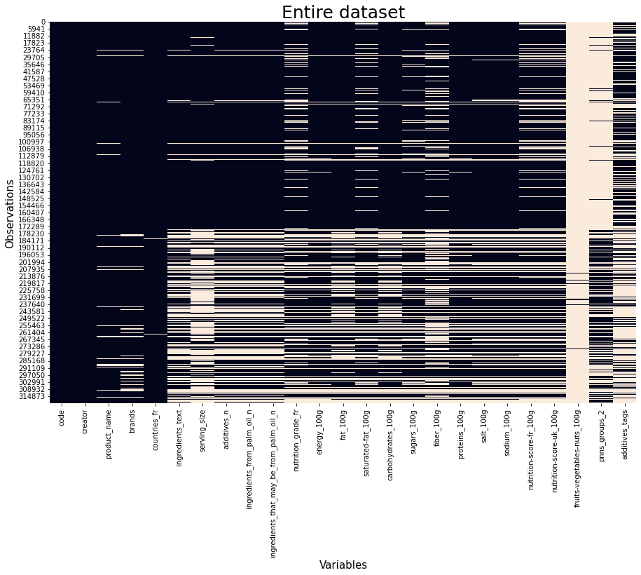
We observe lots of NaNs. However, fewer columns are selected and data analysis can be done.
First, we start with a data description in order to better understand the data.
Describing dataPermalink
df_selected.describe()
| additives_n | ingredients_from_palm_oil_n | ingredients_that_may_be_from_palm_oil_n | energy_100g | fat_100g | saturated-fat_100g | carbohydrates_100g | sugars_100g | fiber_100g | proteins_100g | salt_100g | sodium_100g | nutrition-score-fr_100g | nutrition-score-uk_100g | fruits-vegetables-nuts_100g | |
|---|---|---|---|---|---|---|---|---|---|---|---|---|---|---|---|
| count | 248939.000000 | 248939.000000 | 248939.000000 | 2.611130e+05 | 243891.000000 | 229554.000000 | 243588.000000 | 244971.000000 | 200886.000000 | 259922.000000 | 255510.000000 | 255463.000000 | 221210.000000 | 221210.000000 | 3036.000000 |
| mean | 1.936024 | 0.019659 | 0.055246 | 1.141915e+03 | 12.730379 | 5.129932 | 32.073981 | 16.003484 | 2.862111 | 7.075940 | 2.028624 | 0.798815 | 9.165535 | 9.058049 | 31.458587 |
| std | 2.502019 | 0.140524 | 0.269207 | 6.447154e+03 | 17.578747 | 8.014238 | 29.731719 | 22.327284 | 12.867578 | 8.409054 | 128.269454 | 50.504428 | 9.055903 | 9.183589 | 31.967918 |
| min | 0.000000 | 0.000000 | 0.000000 | 0.000000e+00 | 0.000000 | 0.000000 | 0.000000 | -17.860000 | -6.700000 | -800.000000 | 0.000000 | 0.000000 | -15.000000 | -15.000000 | 0.000000 |
| 25% | 0.000000 | 0.000000 | 0.000000 | 3.770000e+02 | 0.000000 | 0.000000 | 6.000000 | 1.300000 | 0.000000 | 0.700000 | 0.063500 | 0.025000 | 1.000000 | 1.000000 | 0.000000 |
| 50% | 1.000000 | 0.000000 | 0.000000 | 1.100000e+03 | 5.000000 | 1.790000 | 20.600000 | 5.710000 | 1.500000 | 4.760000 | 0.581660 | 0.229000 | 10.000000 | 9.000000 | 23.000000 |
| 75% | 3.000000 | 0.000000 | 0.000000 | 1.674000e+03 | 20.000000 | 7.140000 | 58.330000 | 24.000000 | 3.600000 | 10.000000 | 1.374140 | 0.541000 | 16.000000 | 16.000000 | 51.000000 |
| max | 31.000000 | 2.000000 | 6.000000 | 3.251373e+06 | 714.290000 | 550.000000 | 2916.670000 | 3520.000000 | 5380.000000 | 430.000000 | 64312.800000 | 25320.000000 | 40.000000 | 40.000000 | 100.000000 |
The mean, standard deviation, minimum and maximum values as well as the quantiles are calculated for the numerical variables. It is easy to identify outliers in the maximum and minimum values. It is hoped that these issues will be addressed in the future.
df_selected.describe(include=[object])
| code | creator | product_name | brands | countries_fr | ingredients_text | serving_size | nutrition_grade_fr | pnns_groups_2 | additives_tags | |
|---|---|---|---|---|---|---|---|---|---|---|
| count | 320749 | 320770 | 303010 | 292360 | 320492 | 248962 | 211331 | 221210 | 94491 | 154680 |
| unique | 320749 | 3535 | 221347 | 58784 | 722 | 205520 | 25423 | 5 | 42 | 41537 |
| top | 0000000003087 | usda-ndb-import | Ice Cream | Carrefour | États-Unis | Carbonated water, natural flavor. | 240 ml (8 fl oz) | d | unknown | en:e322 |
| freq | 1 | 169868 | 410 | 2978 | 172998 | 222 | 5496 | 62763 | 22624 | 8264 |
In categorical variables, the count, unique values, most commonly used, and frequency can be gathered. In future analyses, the code can be omitted since it is a unique value. Nevertheless, it is used to detect duplicates.
# afficher les valeurs unique pour chaque variable
df_selected.nunique()
code                                       320749
creator                                      3535
product_name                               221347
brands                                      58784
countries_fr                                  722
ingredients_text                           205520
serving_size                                25423
additives_n                                    31
ingredients_from_palm_oil_n                     3
ingredients_that_may_be_from_palm_oil_n         7
nutrition_grade_fr                              5
energy_100g                                  3997
fat_100g                                     3378
saturated-fat_100g                           2197
carbohydrates_100g                           5416
sugars_100g                                  4068
fiber_100g                                   1016
proteins_100g                                2503
salt_100g                                    5586
sodium_100g                                  5291
nutrition-score-fr_100g                        55
nutrition-score-uk_100g                        55
fruits-vegetables-nuts_100g                   333
pnns_groups_2                                  42
additives_tags                              41537
dtype: int64
df_selected.isna().mean().sort_values(ascending=True)
creator                                    0.000006
code                                       0.000072
countries_fr                               0.000873
product_name                               0.055373
brands                                     0.088574
energy_100g                                0.185986
proteins_100g                              0.189699
salt_100g                                  0.203453
sodium_100g                                0.203599
ingredients_text                           0.223866
additives_n                                0.223938
ingredients_from_palm_oil_n                0.223938
ingredients_that_may_be_from_palm_oil_n    0.223938
sugars_100g                                0.236308
fat_100g                                   0.239675
carbohydrates_100g                         0.240620
saturated-fat_100g                         0.284370
nutrition_grade_fr                         0.310382
nutrition-score-fr_100g                    0.310382
nutrition-score-uk_100g                    0.310382
serving_size                               0.341180
fiber_100g                                 0.373742
additives_tags                             0.517788
pnns_groups_2                              0.705426
fruits-vegetables-nuts_100g                0.990535
dtype: float64
Data cleaningPermalink
The next step is to clean up the data. Data quality and reliability are improved by identifying, correcting, and removing errors, inconsistencies, and inaccuracies. In this process, problems such as missing or duplicate data, incorrect data formatting, outliers, and inconsistencies in the data relationships are identified and resolved. In data preparation and analysis, data cleaning ensures that the data used in a study is accurate, complete, and reliable. Cleansing data is intended to produce high-quality data that can be analyzed in a reliable and meaningful manner.
Quantitative variablesPermalink
Let us look at our quantitative variables. They are also known as numerical variables. This are types of variables in statistics that represent measurable quantities or numerical values. Quantitative variables are typically measured using numerical scales or units of measurement.
Elimination code is NaNPermalink
First, we delete all the rows where code variable does not have a value.
df_selected = df_selected[~df_selected.code.isna()]
Verify duplicates by codePermalink
Next, we verify the duplicates for the codevariable.
## verifié les valeurs dupliqué sur le même code
df_selected.duplicated(['code']).sum()
0
We see that there are no duplicates for this variable.
Dropping the feature codePermalink
Finally, we drop the variable code that does not serve us anymore.
df_selected.drop(['code'], inplace=True, axis=1)
Delete observations with empty nutritionists valuePermalink
The observation with an empty nutritionists value has been deleted.
df_selected = df_selected[~(df_selected.energy_100g.isna() & df_selected.proteins_100g.isna() & df_selected.sugars_100g.isna() & df_selected.fat_100g.isna() &
           df_selected['saturated-fat_100g'].isna() & df_selected.fiber_100g.isna() & df_selected.sodium_100g.isna() & df_selected['fruits-vegetables-nuts_100g'].isna())]
Identifying and correcting outliersPermalink
Here, we identify and delete outliers. Nutrition that is negative or larger than 100g are outliers, and we do not consider them.
mask = ~((df_selected.fiber_100g<0) | (df_selected.fiber_100g>100) |
         (df_selected.salt_100g<0) | (df_selected.salt_100g>100) |
         (df_selected['proteins_100g']<0) | (df_selected['proteins_100g']>100) |
         (df_selected['sugars_100g']<0) | (df_selected['sugars_100g']>100)
        );
df_selected = df_selected[mask];
Additionally, foods contain protein, fat, and carbohydrates. In total, we should not have more than 100 grams. In such a context, we also identify some outliers and discard them.
cols = [
    'proteins_100g',
    'fat_100g',
    'carbohydrates_100g'
    ]
df_selected['sum_on_g'] = df_selected[cols].abs().sum(axis=1)
df_selected['is_outlier'] = df_selected.sum_on_g>100

df_selected = df_selected[df_selected.is_outlier==False];

df_selected.drop(['sum_on_g', 'is_outlier'], inplace=True, axis=1);
Fill NaNPermalink
- First we set
_100gnumerical variables with 0 if they are not specified - Next, for
nutrition_grade_frwe set from ‘a’ to ‘e’ values, using the knowledge fromnutrition-score-fr_100g - energy_100g - Data entry in OpenFood can be difficult and complex, so users may confuse kJ and kcal when introducing the dataset. Calculate the total energy in kcal for all the values (17 proteins, 17 carbohydrates, and 39 fats)
- filling the additive counting variables with 0 if they are not specified
cols = []
for col in df_selected.columns:
    if col.endswith('_100g') & ('nutrition-score' not in col) & ('nutrition-grade' not in col) & (col != 'energy_100g') :
        cols.append(col)
df_selected[cols] = df_selected[cols].fillna(value=0)
Next, we calculate the energy value and set it.
# 1 calorie vaut 180/43 soit 4.1860465116 Joules que nous arrondirons à 4,186 Joules.
# 1000 calories = 1 Kilocalorie = 1 kcal
df_selected['energy_100g'] = 17*df_selected.proteins_100g + 17*df_selected.carbohydrates_100g + 39*df_selected.fat_100g
Now, we fill the NaN values with 0.
df_selected['additives_n'] = df_selected['additives_n'].fillna(value=0)
df_selected['ingredients_from_palm_oil_n'] = df_selected['ingredients_from_palm_oil_n'].fillna(value=0)
df_selected['ingredients_that_may_be_from_palm_oil_n'] = df_selected['ingredients_that_may_be_from_palm_oil_n'].fillna(value=0)
Minimum and maximum of nutriscorePermalink
(df_selected['nutrition-score-fr_100g'].min(), df_selected['nutrition-score-fr_100g'].max())
(-15.0, 40.0)
(df_selected['nutrition-score-uk_100g'].min(), df_selected['nutrition-score-uk_100g'].max())
(-15.0, 36.0)
Qualitative variablesPermalink
Qualitative variables, also known as categorical variables, are types of variables in statistics that represent qualities or characteristics that cannot be measured numerically. These variables are typically represented by non-numeric data or labels such as colors, names, types, or categories.
Creation of variables by taking top valuesPermalink
def create_top(df, col, nr_top):
    col_name = '{0}_top{1}'.format(col , nr_top)
    ll = list(df[col].value_counts().head(5).index)
    df[col_name] = df[col]
    df.loc[~(df[col_name].isin(ll)),col_5] = 'Autre'
For example, we take two variables: creator and countries_fr. We want to select the top 5 values, and for the rest, we will name Autre. In this way, we can see the top values.
take_top_5_col = ['creator', 'countries_fr']

for col in take_top_5_col:
    create_top(df_selected, col, 5)
The same thing we do for the product_name. Here we want to see the top 10 products.
take_top_10_col = ['product_name']

for col in take_top_10_col:
    create_top(df_selected, col, 10)
Clean countries_fr variablePermalink
The : character can be found in the values of countries_fr (ex: ‘en:Tunisie’ and ‘Tunisie.’ should be the same). We need to remove this and make countries have the same name.
df_selected.countries_fr = df_selected.countries_fr.str.replace('en:', '')
df_selected.countries_fr = df_selected.countries_fr.str.replace('es:', '')
df_selected.countries_fr = df_selected.countries_fr.str.replace('de:', '')
df_selected.countries_fr = df_selected.countries_fr.str.replace('ar:', '')
df_selected.countries_fr = df_selected.countries_fr.str.replace('nl:', '')
df_selected.countries_fr = df_selected.countries_fr.str.replace('xx:', '')


df_selected.loc[(df_selected.countries_fr.str.lower() == 'royaume-uni') | (df_selected.countries_fr.str.lower() == 'Angleterre'), 'countries_fr'] = 'Royaume-Uni'
df_selected.loc[(df_selected.countries_fr.str.lower() == '77-provins') | (df_selected.countries_fr.str.lower() == 'Aix-en-provence'), 'countries_fr'] = 'France'
CorrelationPermalink
Correlation between two variables refers to the statistical relationship between them. Specifically, correlation measures the degree to which two variables are related or vary together.
In general, there are two types of correlation: positive and negative. A positive correlation exists when an increase in one variable is associated with an increase in the other variable, while a negative correlation exists when an increase in one variable is associated with a decrease in the other variable.
The strength of the correlation is measured by the correlation coefficient, which ranges from -1 to 1. A correlation coefficient of -1 indicates a perfect negative correlation, 0 indicates no correlation, and 1 indicates a perfect positive correlation.
Correlation is often used in statistical analysis to understand the relationship between two variables and to make predictions about one variable based on the other. However, correlation does not necessarily imply causation, and other factors may be influencing the relationship between the two variables. Therefore, the correlation should be interpreted with caution and further analysis should be conducted to establish causation.
Between 2 quantitative variablesPermalink
plot_correlation(df_selected)
| additives_n | ingredients_from_palm_oil_n | ingredients_that_may_be_from_palm_oil_n | energy_100g | fat_100g | saturated-fat_100g | carbohydrates_100g | sugars_100g | fiber_100g | proteins_100g | salt_100g | sodium_100g | nutrition-score-fr_100g | nutrition-score-uk_100g | fruits-vegetables-nuts_100g | |
|---|---|---|---|---|---|---|---|---|---|---|---|---|---|---|---|
| additives_n | nan | nan | nan | nan | nan | nan | nan | nan | nan | nan | nan | nan | nan | nan | nan |
| ingredients_from_palm_oil_n | 0.120900 | nan | nan | nan | nan | nan | nan | nan | nan | nan | nan | nan | nan | nan | nan |
| ingredients_that_may_be_from_palm_oil_n | 0.288444 | 0.184633 | nan | nan | nan | nan | nan | nan | nan | nan | nan | nan | nan | nan | nan |
| energy_100g | 0.039412 | 0.098584 | 0.031941 | nan | nan | nan | nan | nan | nan | nan | nan | nan | nan | nan | nan |
| fat_100g | -0.078317 | 0.063591 | 0.025512 | 0.802379 | nan | nan | nan | nan | nan | nan | nan | nan | nan | nan | nan |
| saturated-fat_100g | -0.061414 | 0.084041 | 0.030113 | 0.507905 | 0.636419 | nan | nan | nan | nan | nan | nan | nan | nan | nan | nan |
| carbohydrates_100g | 0.200227 | 0.083950 | 0.030712 | 0.540972 | -0.042021 | -0.047544 | nan | nan | nan | nan | nan | nan | nan | nan | nan |
| sugars_100g | 0.146411 | 0.058287 | 0.005414 | 0.274477 | -0.063760 | 0.063558 | 0.617330 | nan | nan | nan | nan | nan | nan | nan | nan |
| fiber_100g | -0.115047 | -0.001547 | -0.035574 | 0.249919 | 0.095830 | 0.004550 | 0.230889 | -0.017901 | nan | nan | nan | nan | nan | nan | nan |
| proteins_100g | -0.101381 | -0.007868 | -0.038991 | 0.277584 | 0.213393 | 0.194014 | -0.093323 | -0.238110 | 0.231642 | nan | nan | nan | nan | nan | nan |
| salt_100g | -0.003864 | -0.005207 | -0.016555 | -0.077246 | -0.046840 | -0.039982 | -0.067531 | -0.091756 | -0.032159 | -0.001990 | nan | nan | nan | nan | nan |
| sodium_100g | -0.003864 | -0.005207 | -0.016555 | -0.077246 | -0.046840 | -0.039983 | -0.067532 | -0.091756 | -0.032159 | -0.001990 | 1.000000 | nan | nan | nan | nan |
| nutrition-score-fr_100g | 0.152258 | 0.111722 | 0.055395 | 0.563106 | 0.533356 | 0.632214 | 0.234830 | 0.467773 | -0.161741 | 0.108323 | 0.126733 | 0.126734 | nan | nan | nan |
| nutrition-score-uk_100g | 0.150110 | 0.114145 | 0.056638 | 0.585692 | 0.557287 | 0.649291 | 0.235674 | 0.457226 | -0.155272 | 0.131695 | 0.130602 | 0.130602 | 0.986087 | nan | nan |
| fruits-vegetables-nuts_100g | -0.013594 | -0.006479 | -0.001290 | -0.051571 | -0.039096 | -0.037375 | -0.021815 | 0.016174 | -0.015843 | -0.047305 | -0.015122 | -0.015122 | -0.041717 | -0.058165 | nan |
st.pearsonr(df_selected.fat_100g, df_selected.energy_100g)[0] # coefficient de correlation lineere
np.cov(df_selected.fat_100g, df_selected.energy_100g, ddof=0) # matrice de covariance
0.8023789000889111

array([[2.91999772e+02, 1.15335422e+04],
       [1.15335422e+04, 7.07593613e+05]])
Between 1 quantitative variable and 1 qualitative variable (ANOVA)Permalink
data = get_pandas_catVar_numVar(df_selected, catVar = 'product_name_top10', numVar = 'fat_100g')

# Propriétés graphiques (pas très importantes)
medianprops = {'color':"black"}
meanprops = {'marker':'o', 'markeredgecolor':'black',
            'markerfacecolor':'firebrick'}

plt.figure(figsize=(20,8));
b = sns.boxplot(x="variable", y="value", data=pd.melt(data), showfliers = False,  showmeans=True, medianprops=medianprops, meanprops=meanprops);
plt.title('Top 10: product_name / fat_100g', fontsize=20);
plt.xlabel('Variable values', fontsize=15);
plt.ylabel('Values', fontsize=15);
plt.show();
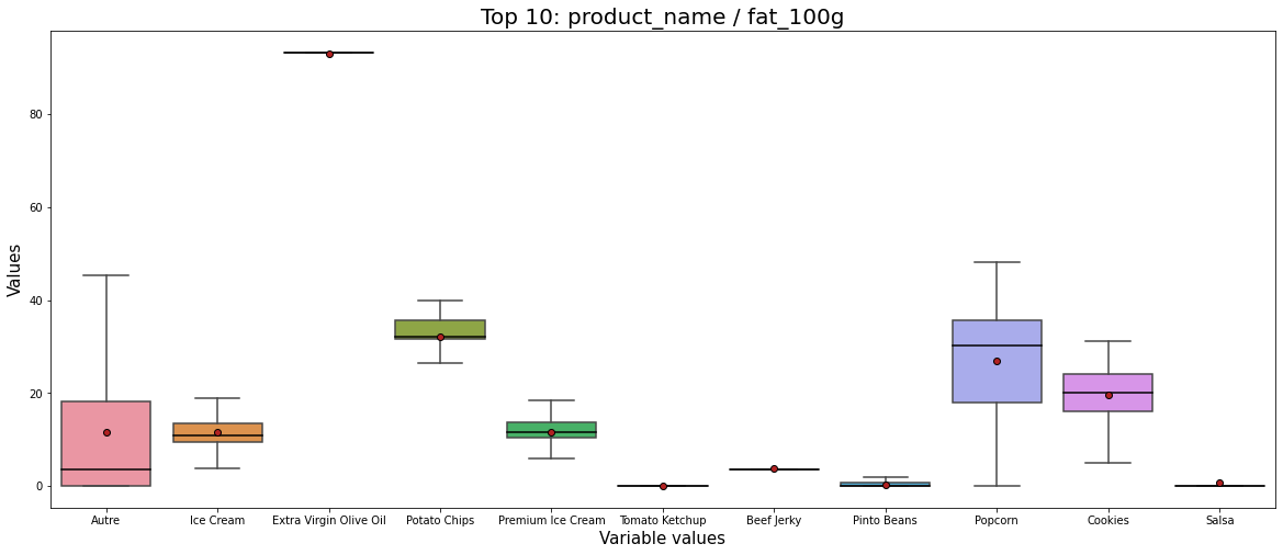
By analyzing Figure 4 we can say:
- The fat is different from one product to other.
- For instance, the fat for Potato chips, Cookies, and Popcorn is more considerable and more dispersed than those of salsa, and pinto beans.
- The product that contains the biggest fat is Extra Virgin Olive Oil which is logical.
We shall say here that according to our application, some of these products could be omitted by our users. For example, if we want to eat cookies that have less than 30 fat, that means not all cookies are permitted, and those will not be selected.
data = get_pandas_catVar_numVar(df_selected, catVar = 'product_name_top10', numVar = 'energy_100g')

# Propriétés graphiques (pas très importantes)
medianprops = {'color':"black"}
meanprops = {'marker':'o', 'markeredgecolor':'black',
            'markerfacecolor':'firebrick'}

plt.figure(figsize=(20,8));
b = sns.boxplot(x="variable", y="value", data=pd.melt(data), showfliers = False);
plt.title('Top 10: product_name / energy_100g', fontsize=20);
plt.xlabel('Variable values', fontsize=15);
plt.ylabel('Values', fontsize=15);
plt.show();
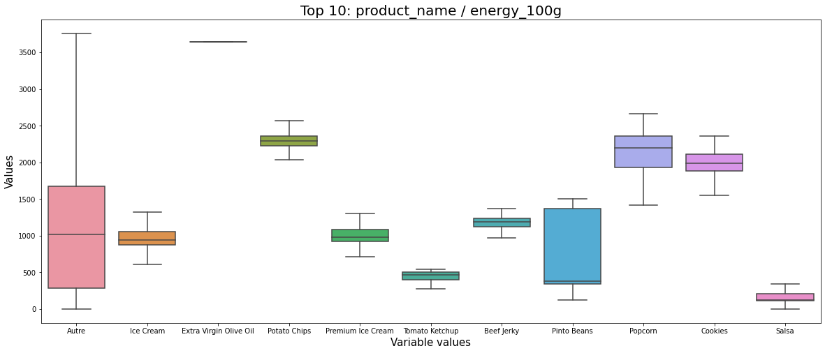
By analyzing Figure 5 we can say:
- Somehow the energy is similar to the fat. The higher fat produces higher energy products. However, they are more dispersed on the energy variable than on the fat variable.
- Having a standing profession high caloric products should be evited. For example, tacking cookies with preferred less kcal for persons with the sitting profession.
By analyzing the correlation of one quantitative and one qualitative variable we look for the eta squared coefficient. Suppose Y is a categorical variable and X is a numerical variable, we look at the correlation between these variables with eta_squared = Total_variance/Inclass_variance. If eta_squared = 0, it means that the class averages are all equal. There is therefore no a priori relationship between the variables Y and X. On the contrary, if eta_squared = 1, this means that the averages per class are very different, and each class is made up of identical values: there is therefore a priori a relationship between the variables Y and X.
eta_squared(df_selected, 'product_name_top10', 'energy_100g')
0.015498074324149612
eta_squared(df_selected, 'product_name_top10', 'fat_100g')
0.029213633935751267
eta_squared(df_selected[~df_selected.nutrition_grade_fr.isna()], 'nutrition_grade_fr', 'energy_100g')
0.2982499803324311
eta_squared(df_selected[~df_selected.nutrition_grade_fr.isna()], 'nutrition_grade_fr', 'fat_100g')
0.2618975105793661
By computing, some of the eta squared we can say that the nutrition grade has a correlation with the fat and energy variables.
Between two qualitatives variablesPermalink
Let us pose a question. Do you have the same products in different states?
X = "product_name_top10"
Y = "countries_fr_top5"

cont = df_selected[[X,Y]].pivot_table(index=X,columns=Y,aggfunc=len,margins=True,margins_name="Total")

plt.figure(figsize=(20,8));
sns.heatmap(cont, cmap="YlGnBu", annot=True, fmt='.1f')
plt.title('Top 10 produits dans top 5 états', fontsize=20);
plt.xlabel('Top 5 états', fontsize=15);
plt.ylabel('Top 10 produits', fontsize=15);
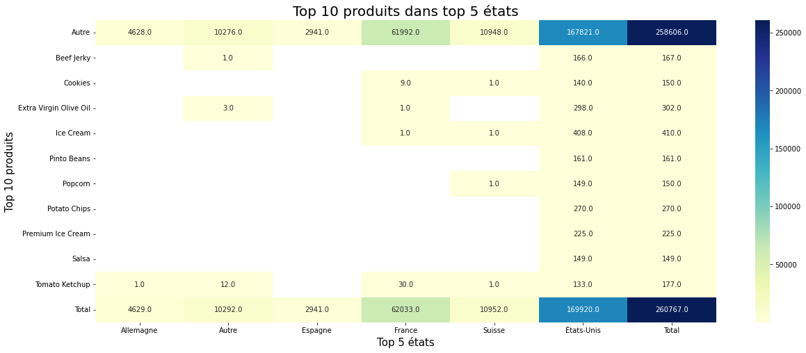
By analyzing Figure 6 we can say that:
- the top ten products are all observed in the US.
- France is the second country that has most of the observed products.
Data AnalysisPermalink
Univariate analysePermalink
Densities of nutritional variablesPermalink
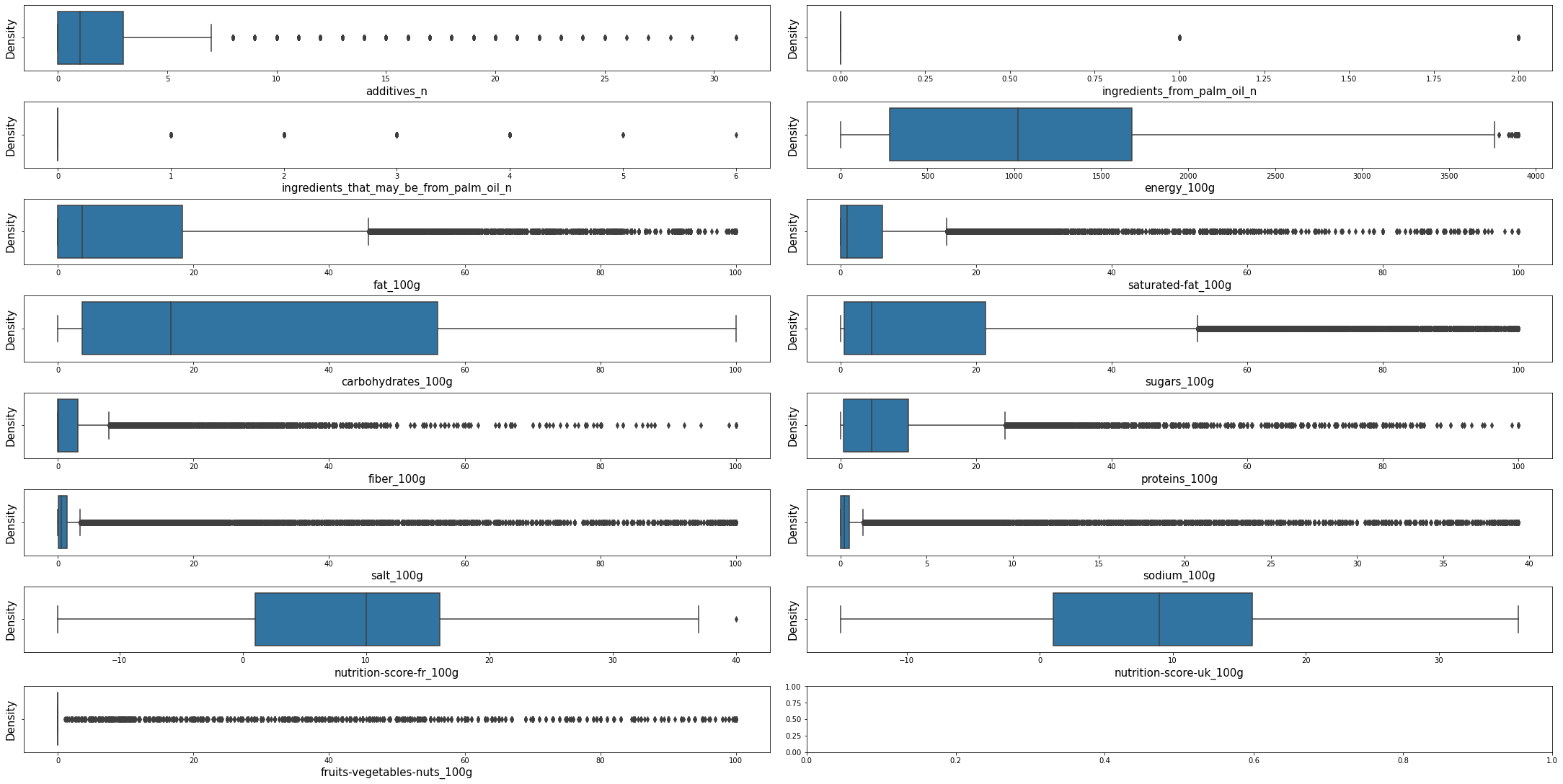
plot_density(df_selected, dt = DensityTypes.Boxplot) #dt = DensityTypes.Density
Visualizing some of the top variables valuesPermalink
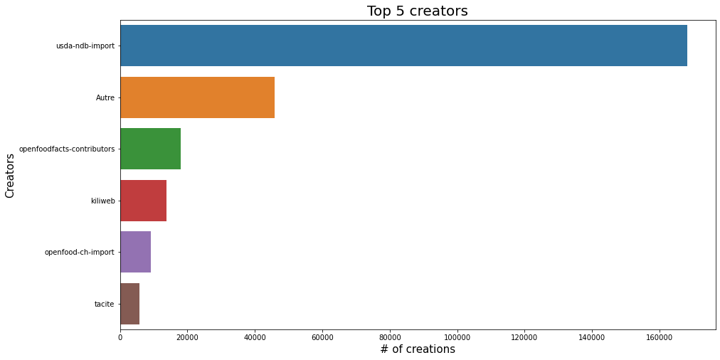
plt.figure(figsize=(15,8))
sns.barplot(x=df_selected.creator_top5.value_counts(), y=df_selected.creator_top5.value_counts().index, data=df_selected);
plt.title('Top 5 creators', fontsize=20);
plt.xlabel('# of creations', fontsize=15);
plt.ylabel('Creators', fontsize=15);
plt.show();
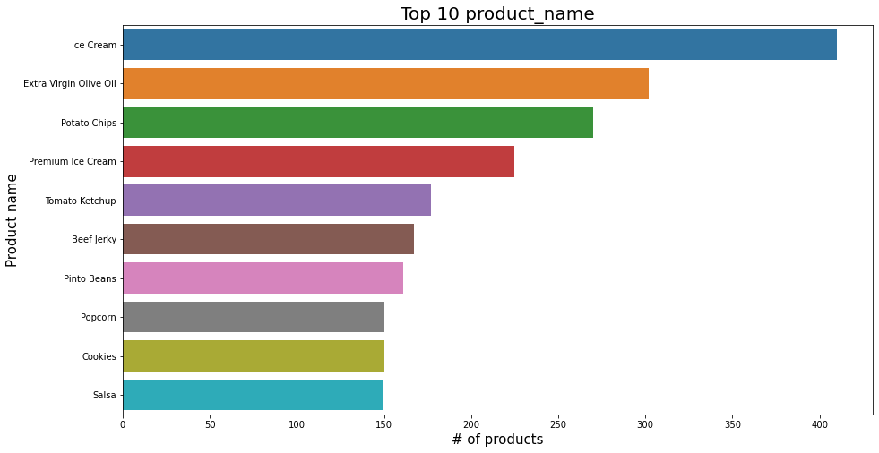
plt.figure(figsize=(15,8))
sns.barplot(x=df_selected.product_name.value_counts().head(10), y=df_selected.product_name.value_counts().head(10).index, data=df_selected);
plt.title('Top 10 product_name', fontsize=20);
plt.xlabel('# of products', fontsize=15);
plt.ylabel('Product name', fontsize=15);
plt.show();
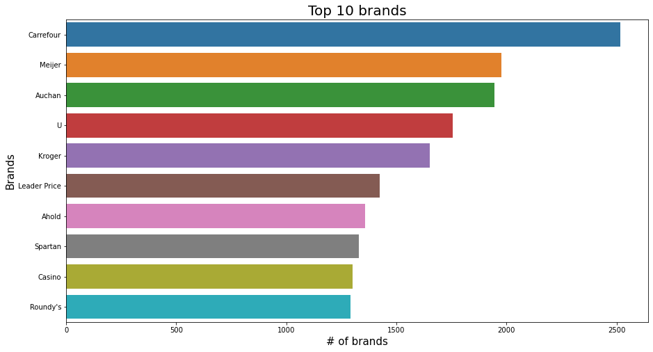
plt.figure(figsize=(15,8))
sns.barplot(x=df_selected.brands.value_counts().head(10), y=df_selected.brands.value_counts().head(10).index, data=df_selected);
plt.title('Top 10 brands', fontsize=20);
plt.xlabel('# of brands', fontsize=15);
plt.ylabel('Brands', fontsize=15);
plt.show();
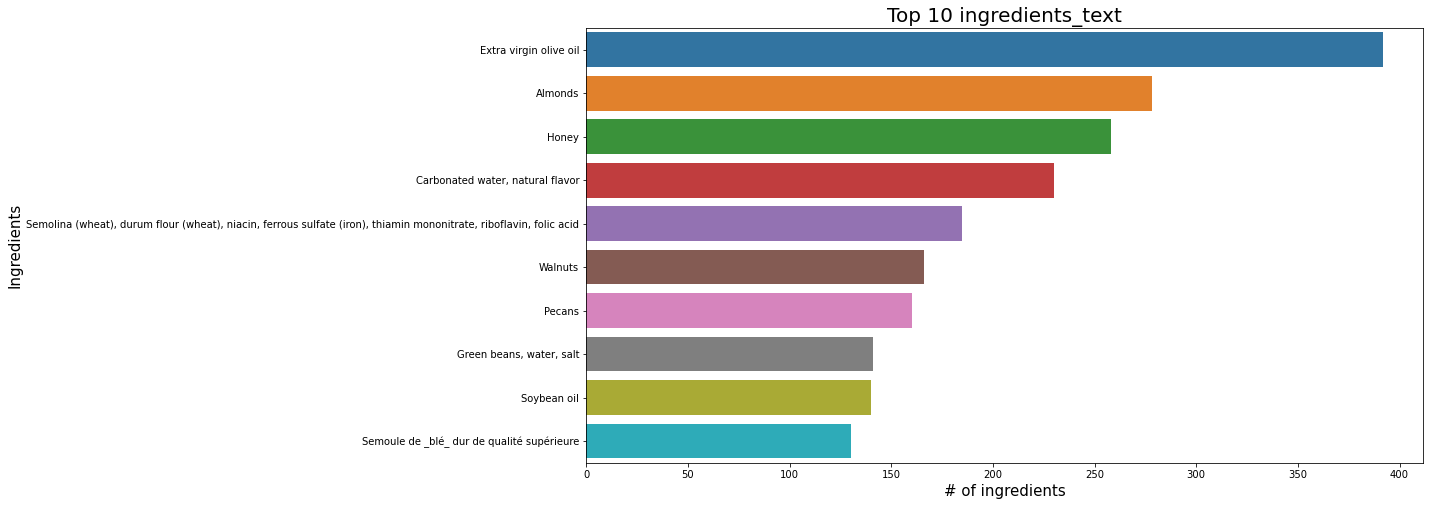
plt.figure(figsize=(15,8))
sns.barplot(x=df_selected.ingredients_text.value_counts().head(10), y=df_selected.ingredients_text.value_counts().head(10).index, data=df_selected);
plt.title('Top 10 ingredients_text', fontsize=20);
plt.xlabel('# of ingredients', fontsize=15);
plt.ylabel('Ingredients', fontsize=15);
plt.show();
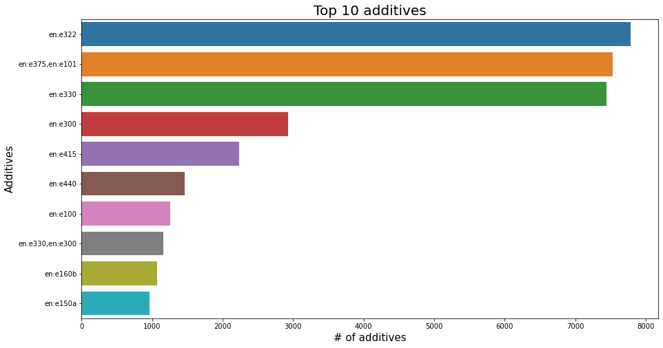
plt.figure(figsize=(15,8))
sns.barplot(x=df_selected.additives_tags.value_counts().head(10), y=df_selected.additives_tags.value_counts().head(10).index, data=df_selected);
plt.title('Top 10 additives', fontsize=20);
plt.xlabel('# of additives', fontsize=15);
plt.ylabel('Additives', fontsize=15);
plt.show();
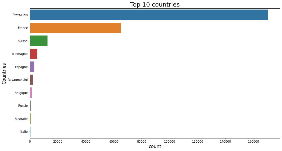
df1 =  df_selected.countries_fr.str.split(',', expand=True).melt(var_name='columns', value_name='values');
df2 = pd.crosstab(index=df1['values'], columns=df1['columns'], margins=True).All.drop('All').sort_values(ascending = False).head(10);
df2 = df2.to_frame();
#Using reset_index, inplace=True
df2.reset_index(inplace=True);

plt.figure(figsize=(15,8));
sns.barplot(y='values', x='All', data=df2);
plt.title('Top 10 countries', fontsize=20);
plt.xlabel('count', fontsize=15);
plt.ylabel('Countries', fontsize=15);
plt.show();

del df1, df2;
plot_words(df, 'countries_fr')

Distribution of nutriscore_gradePermalink
plt.figure(figsize=(15,8))
df_selected.nutrition_grade_fr.value_counts().plot.pie(autopct="%.1f%%");
plt.title('Nutriscore grade', fontsize=20);
plt.ylabel('');
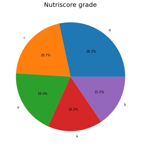
nutriscore_grade distribution.
Multivariate analysisPermalink
cols = ['energy_100g', 'fat_100g', 'saturated-fat_100g', 'carbohydrates_100g', 'sugars_100g',
  'salt_100g', 'nutrition_grade_fr']
d = df_selected[(~df_selected['nutrition_grade_fr'].isna()) & (~df_selected['nutrition-score-fr_100g'].isna())][cols].sample(10000)

sns.pairplot(data=d, hue="nutrition_grade_fr", hue_order=['e','d','c','b','a'],
             plot_kws = {'s': 10}, corner=True)
del d
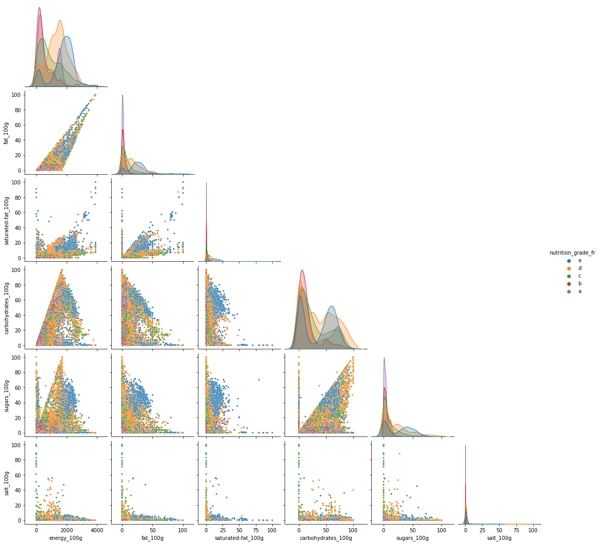
Analyzing Figure 15 we can say:
The level of fats and that of saturated fats penalizes the nutriscore.
Other nutrition compositions affect less the nutriscore. However, some effects can be observed. This difference can be due to the food categories.
Some foods are rich in caloric energy having a good nutrition grade:
- A high nutrition grade of ‘a’ and ‘b’ with energy in the range of 1500 can be observed with fat smaller than 20
- A high nutrition grade of ‘a’ and ‘b’ with energy in a range of 3000 can be observed with very less saturated fat that is less than 10.
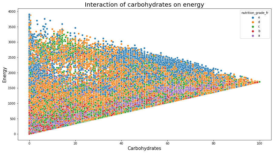
- We observe foods rich in carbohydrates that have a good nutrition score having more than 2000 in energy.
These can be also seen in the following 3 figures.
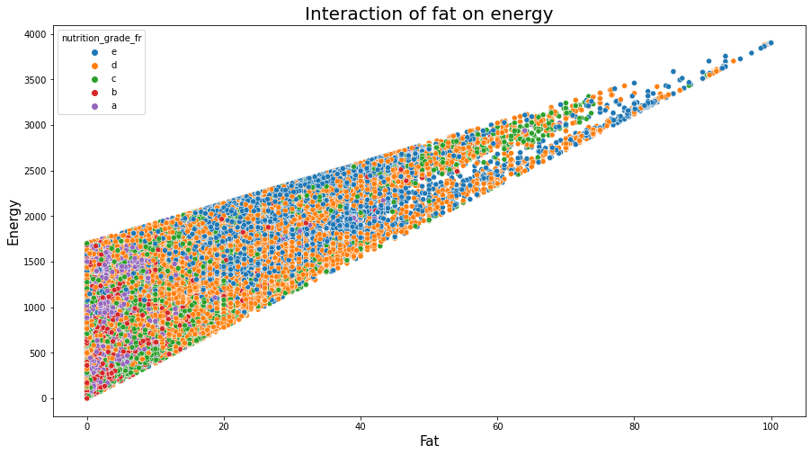
plt.figure(figsize=(15,8));
sns.scatterplot(data=df_selected, x="fat_100g", y="energy_100g", hue="nutrition_grade_fr", hue_order=['e','d','c','b','a'])
plt.title('Interaction of fat on energy', fontsize=20);
plt.xlabel('Fat', fontsize=15);
plt.ylabel('Energy', fontsize=15);
plt.show();
plt.figure(figsize=(15,8));
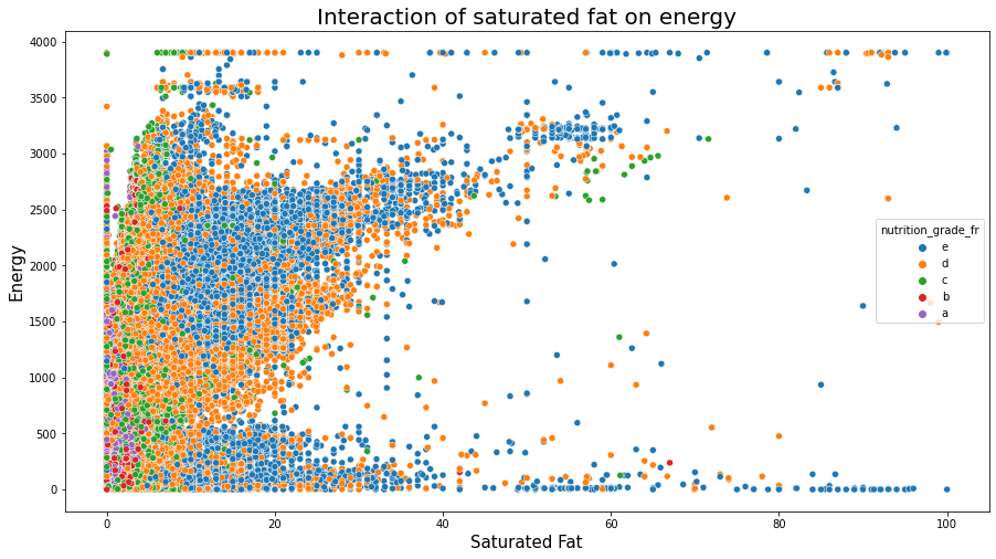
sns.scatterplot(data=df_selected, x="saturated-fat_100g", y="energy_100g", hue="nutrition_grade_fr", hue_order=['e','d','c','b','a'])
plt.title('Interaction of saturated fat on energy', fontsize=20);
plt.xlabel('Saturated Fat', fontsize=15);
plt.ylabel('Energy', fontsize=15);
plt.show();
plt.figure(figsize=(15,8));
sns.scatterplot(data=df_selected, x="carbohydrates_100g", y="energy_100g", hue="nutrition_grade_fr", hue_order=['e','d','c','b','a'])
plt.title('Interaction of carbohydrates on energy', fontsize=20);
plt.xlabel('Carbohydrates', fontsize=15);
plt.ylabel('Energy', fontsize=15);
plt.show();
plt.figure(figsize=(15,8));
sns.boxplot(x="nutrition_grade_fr", y="energy_100g", data=df_selected, showfliers = False, order = ['a', 'b', 'c', 'd', 'e'])
plt.title('Nutrition grade distributions/ Energy', fontsize=20);
plt.xlabel('Nutrition grade', fontsize=15);
plt.ylabel('Energy', fontsize=15);
plt.show();
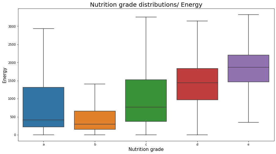
nutrition_grade_fr distributions over the energy_100g variable
plt.figure(figsize=(15,8));
sns.boxplot(x="nutrition_grade_fr", y="fat_100g", data=df_selected, showfliers = False, order = ['a', 'b', 'c', 'd', 'e'])
plt.title('Nutrition grade distributions/ fat_100g', fontsize=20);
plt.xlabel('Nutrition grade', fontsize=15);
plt.ylabel('Fat', fontsize=15);
plt.show();
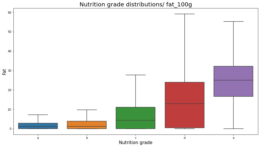
nutrition_grade_fr distributions over the fat_100g variable
Note that foods with different nutrition_grade_fr can have relatively equal high energies. But preferring good foods (with nutrition_grade_fr ‘a’ and ‘b’) we are likely to eat foods with less energy. The same thing we observe in fat foods, where preferring better foods (with a better nutrition score) we shall choose not fat foods.
Add my_category variablePermalink
plot_words(df_selected, 'pnns_groups_2')
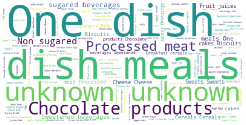
compute_words_freq(df_selected, 'pnns_groups_2', sep=',')
| Word | Frequency | |
|---|---|---|
| 0 | unknown | 12835 |
| 1 | one-dish meals | 4927 |
| 2 | biscuits and cakes | 4018 |
| 3 | cereals | 3701 |
| 4 | sweets | 3587 |
| 5 | cheese | 3516 |
| 6 | milk and yogurt | 2914 |
| 7 | dressings and sauces | 2785 |
| 8 | chocolate products | 2648 |
| 9 | vegetables | 2585 |
| 10 | processed meat | 2548 |
| 11 | non-sugared beverages | 2242 |
| 12 | fish and seafood | 2052 |
| 13 | sweetened beverages | 1952 |
| 14 | appetizers | 1880 |
| 15 | fruit juices | 1729 |
| 16 | bread | 1590 |
| 17 | fats | 1342 |
| 18 | breakfast cereals | 1310 |
| 19 | fruits | 1297 |
| 20 | meat | 1150 |
| 21 | legumes | 754 |
| 22 | dairy desserts | 726 |
| 23 | ice cream | 647 |
| 24 | sandwich | 640 |
| 25 | nuts | 565 |
| 26 | pizza pies and quiche | 464 |
| 27 | soups | 463 |
| 28 | dried fruits | 410 |
| 29 | pastries | 403 |
| 30 | fruit nectars | 342 |
| 31 | artificially sweetened beverages | 255 |
| 32 | eggs | 186 |
| 33 | alcoholic beverages | 155 |
| 34 | potatoes | 96 |
| 35 | tripe dishes | 49 |
| 36 | salty and fatty products | 19 |
categories ={
    'cheese' : ['cheese'],
    'appetizer' : ['appetizers', 'nuts', 'salty and fatty products', 'dressings and sauces'],
    'melange': ['soups', 'sandwich', 'pizza pies and quiche'],
    'juice' : ['fruit juices', 'fruit nectars'],
    'plants' : ['legumes', 'legume', 'fruits', 'Fruit', 'vegetables', 'dried fruits'],
    'sweet' : ['sweets', 'biscuits and cakes', 'chocolate products', 'dairy desserts'],
    'feculent' : ['cereals', 'bread', 'pastries', 'potatoes', 'breakfast cereals' ],
    'beverage' : ['non-sugared beverages', 'artificially sweetened beverages', 'alcoholic beverages', 'sweetened beverages'],
    'meat_fish' : ['tripe dishes', 'meat','fish and seafood', 'processed meat', 'eggs'],
    'fats' : ['fats'],
    'milk' : ['milk and yogurt', 'ice cream'],
}

def replace(df, col, key, val):
    m = [v == key for v in df[col]]
    df.loc[m, col] = val
    return df

df_selected2 = df_selected[~df_selected.pnns_groups_2.isna()]
plot_data(df_selected2)

df_selected2['my_categoty'] = df_selected2['pnns_groups_2'].str.lower();
for new_value, old_value in categories.items():
    #print(old_value)
    df_selected['my_categoty'] = df_selected['my_categoty'].replace(old_value, new_value);
    #df_selected2['my_categoty'] = df_selected2['my_categoty'].replace(['appetizers', 'nuts', 'salty and fatty products', 'dressings and sauces'], 'appetizer');

plot_words(df_selected, 'my_categoty')
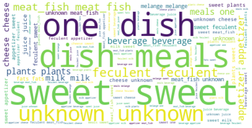
compute_words_freq(df_selected, 'my_categoty')
| Word | Frequency | |
|---|---|---|
| 0 | unknown | 12835 |
| 1 | sweet | 10979 |
| 2 | feculent | 7100 |
| 3 | meat_fish | 5985 |
| 4 | appetizer | 5249 |
| 5 | plants | 5046 |
| 6 | onedish | 4927 |
| 7 | meals | 4927 |
| 8 | beverage | 4604 |
| 9 | milk | 3561 |
| 10 | cheese | 3516 |
| 11 | juice | 2071 |
| 12 | melange | 1567 |
| 13 | fats | 1342 |
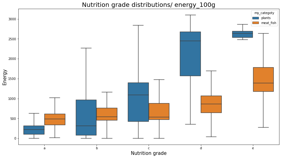
plt.figure(figsize=(15,8));
sns.boxplot(x="nutrition_grade_fr", y="energy_100g", data=df_selected[(df_selected.my_categoty == 'plants') | (df_selected.my_categoty == 'meat_fish')], showfliers = False, order = ['a', 'b', 'c', 'd', 'e'], hue =  'my_categoty')
plt.title('Nutrition grade distributions/ energy_100g', fontsize=20);
plt.xlabel('Nutrition grade', fontsize=15);
plt.ylabel('Energy', fontsize=15);
plt.show();
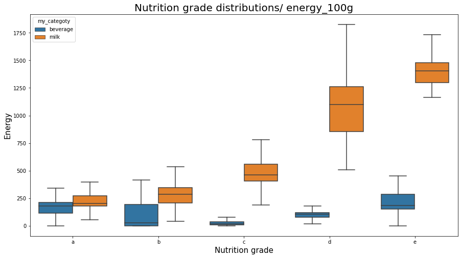
plt.figure(figsize=(15,8));
sns.boxplot(x="nutrition_grade_fr", y="energy_100g", data=df_selected[(df_selected.my_categoty == 'beverage') | (df_selected.my_categoty == 'milk')], showfliers = False, order = ['a', 'b', 'c', 'd', 'e'], hue =  'my_categoty')
plt.title('Nutrition grade distributions/ energy_100g', fontsize=20);
plt.xlabel('Nutrition grade', fontsize=15);
plt.ylabel('Energy', fontsize=15);
plt.show();
Difference between nutriscoresPermalink
Let us now examine if there are some differences between nutri-score-fr_100g and nutriscore-uk-100g.
from sklearn.linear_model import LinearRegression
mask = (~df_selected['nutrition-score-fr_100g'].isna()) & (~df_selected['nutrition-score-uk_100g'].isna())
x=df_selected[mask]['nutrition-score-fr_100g']
y=df_selected[mask]['nutrition-score-uk_100g']

plt.figure(figsize=(15,8));
sns.scatterplot(x,
                y,
                hue = df_selected['my_categoty'],
                legend='full',
                s=100);

plt.title('Nutri score UK vs FR', fontsize=20);
plt.xlabel('nutri score fr 100g', fontsize=15);
plt.ylabel('nutri score uk 100g', fontsize=15);


#linear regression
x = np.array(x).reshape(-1, 1);
y = np.array(y).reshape(-1, 1);

reg = LinearRegression();
model = reg.fit(x, y);
plt.plot(x, model.predict(x),color='k');
plt.show()

print('y=ax with a={}\n score : {}'.format(model.coef_[0], model.score(x, y)));
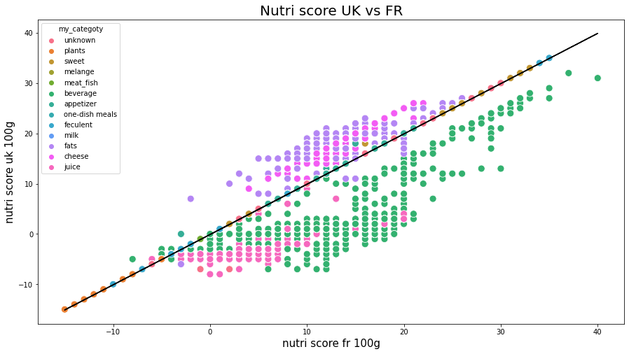
nutrition-score-fr and nutrition-score-uk
 y=ax with a=[1.0000532]
 score : 0.9723672948764118
Nutriscore for the two countries are rather similar, a linear model between them is easily modeled. However, we see some differences in the computation of nutriscore for some categories of products:
- beverage is considered with a smaller nutrition score
- fats are considered with a higher nutrition score
- cheese is considered with a higher nutrition score
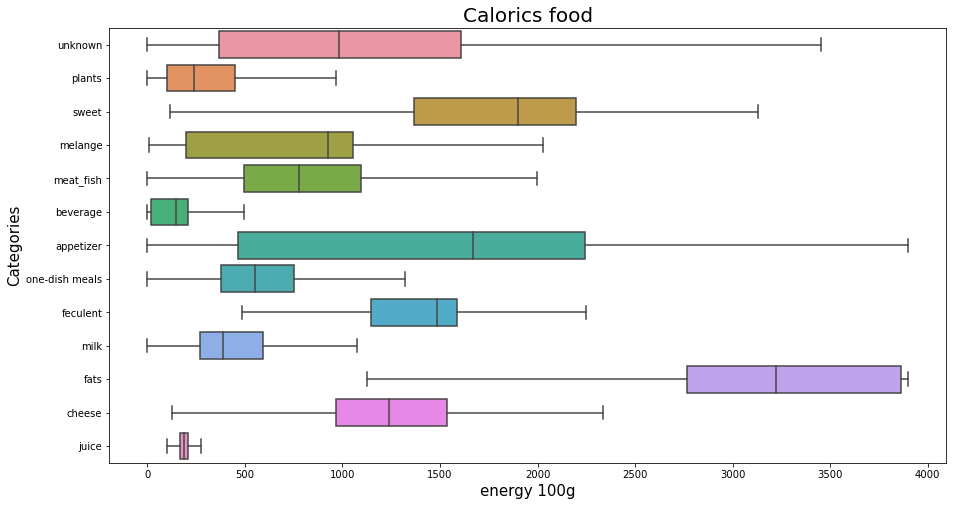
Energy for each category of foods?Permalink
plt.figure(figsize=(15,8));
sns.boxplot(x="energy_100g", y="my_categoty", data=df_selected, orient = 'h', showfliers = False,);
plt.title('Calorics food', fontsize=20);
plt.xlabel('energy 100g', fontsize=15);
plt.ylabel('Categories', fontsize=15);
plt.show();
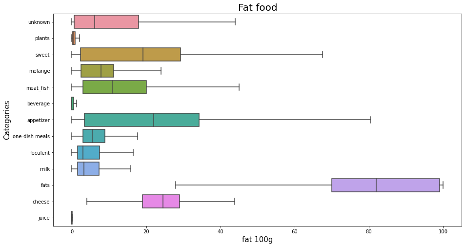
Fat for each category of foods?Permalink
plt.figure(figsize=(15,8));
sns.boxplot(x="fat_100g", y="my_categoty", data=df_selected, orient = 'h', showfliers = False,);
plt.title('Fat food', fontsize=20);
plt.xlabel('fat 100g', fontsize=15);
plt.ylabel('Categories', fontsize=15);
plt.show();
Exploratory analysis with PCAPermalink
PCA allows us to:
- Analyse the variability between individuals, i.e. what are the differences and similarities between individuals.
- Analyse links between variables: what are there groups of variables that are highly correlated with each other that can be grouped into new synthetic variables?
# selection des colonnes à prendre en compte dans l'ACP
columns_acp = []
for c in list(df_selected.columns):
    if c.endswith('_100g'):
        columns_acp.append(c)
df_pca = df_selected[columns_acp]

plot_data(df_pca)
# Preparation des données
from sklearn.impute import SimpleImputer
imp = SimpleImputer(missing_values=np.nan, strategy='mean');
X = np.array(df_pca['nutrition-score-fr_100g']).reshape(-1, 1);
imp.fit(X);
df_pca['nutrition-score-fr_100g'] = imp.transform(X);

X = np.array(df_pca['nutrition-score-uk_100g']).reshape(-1, 1);
imp.fit(X);
df_pca['nutrition-score-uk_100g'] = imp.transform(X);
#del X
X = df_pca.values
names = df_pca.index #["product_name"] # ou data.index pour avoir les intitulés
features = df_pca.columns

# Centrage et Réduction
std_scale = preprocessing.StandardScaler().fit(X)
X_scaled = std_scale.transform(X)
# choix du nombre de composantes à calculer
n_comp = 6

# Calcul des composantes principales
pca = decomposition.PCA(n_components=n_comp)
pca.fit(X_scaled)

X_projected = pca.fit_transform(X_scaled)


X_projected = pd.DataFrame(X_projected, index = df_pca.index, columns = ['F{0}'.format(i) for i in range(n_comp)])

X_projected
PCA(n_components=6)
| F0 | F1 | F2 | F3 | F4 | F5 | |
|---|---|---|---|---|---|---|
| 1 | 2.969878 | -0.398472 | 0.512247 | 0.170433 | 0.168039 | -1.250576 |
| 2 | -0.119704 | -0.925610 | 0.434700 | 2.543939 | 0.046679 | 0.171516 |
| 3 | 2.309261 | 0.007418 | 2.223656 | 1.584307 | 0.250097 | -0.581340 |
| 4 | 0.002351 | -0.753928 | -0.451536 | 1.405344 | -0.106914 | 0.298048 |
| 5 | 0.858225 | -0.791237 | 0.211521 | 1.907893 | 0.022654 | 0.200782 |
| ... | ... | ... | ... | ... | ... | ... |
| 320756 | 0.157600 | 0.036311 | 0.451537 | -0.319817 | 0.015153 | -1.009554 |
| 320757 | -1.670609 | -0.420981 | 1.782779 | 1.898136 | -0.025061 | 1.269749 |
| 320763 | -2.339713 | -0.139322 | 0.323233 | -0.883152 | -0.164451 | -0.445308 |
| 320768 | -2.492881 | -0.161867 | 0.332084 | -0.887011 | -0.164449 | -0.535805 |
| 320771 | -1.512330 | 0.099590 | 0.084318 | -1.414149 | -0.217476 | -0.020945 |
260767 rows × 6 columns
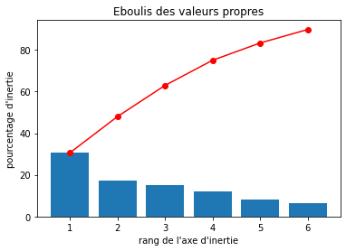
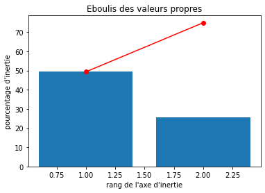
# Eboulis des valeurs propres
display_scree_plot(pca)
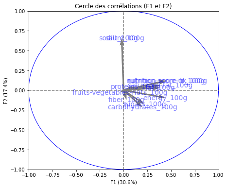
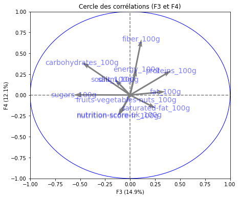
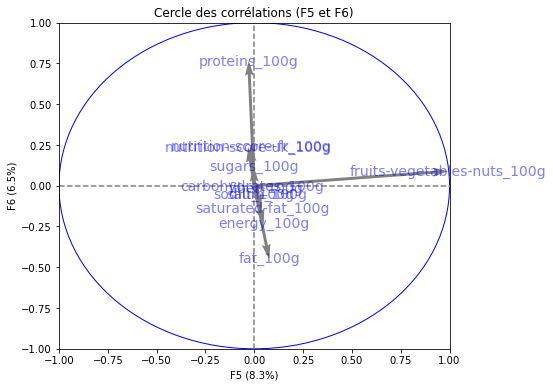
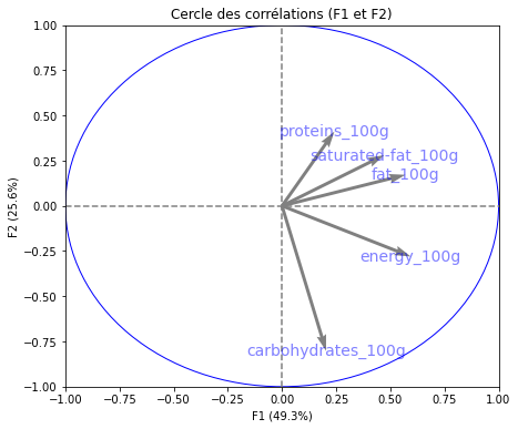
# Cercle des corrélations
pcs = pca.components_
display_circles(pcs, n_comp, pca, [(0,1),(2,3),(4,5)], labels = np.array(features))
Percentages of inertia, also known as the percentage of variance explained or proportion of variance, is a measure of the amount of variation in a dataset that is accounted for by a particular factor or component in a statistical analysis.
In multivariate statistical techniques such as principal component analysis (PCA), correspondence analysis, or factor analysis, percentages of inertia are used to assess the importance of each factor or component. The percentage of inertia is calculated as the proportion of the total variance of the dataset that is explained by a particular factor or component.
For example, in PCA, the first principal component accounts for the largest percentage of variance in the dataset, followed by the second principal component, and so on. The percentage of inertia for each principal component indicates how much of the variance in the dataset is accounted for by that component.
Percentages of inertia are useful in interpreting and visualizing the results of multivariate statistical analyses, as they provide a measure of the relative importance of each factor or component in explaining the variability in the data.
# Projection des individus
X_projected = pca.transform(X_scaled)
display_factorial_planes(X_projected, n_comp, pca, [(0,1),(2,3),(4,5)], alpha = 0.2)
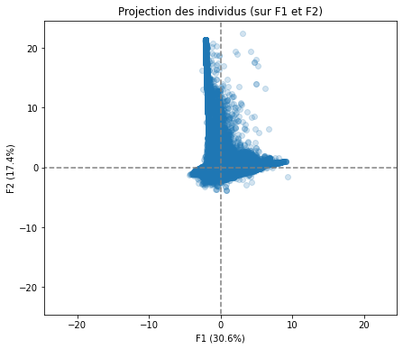
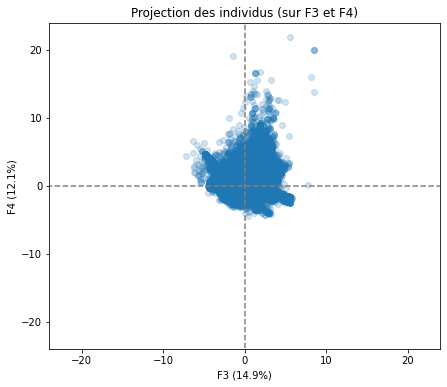
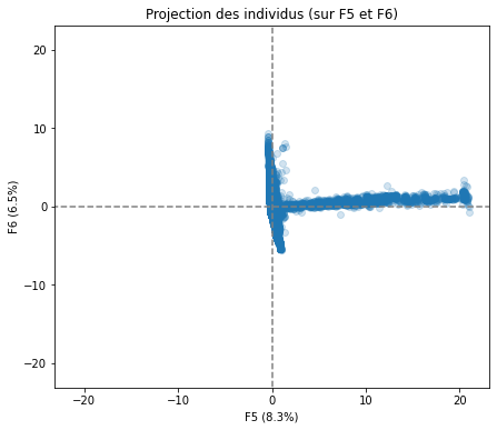
Realizing PCA with 6 composants capturing greater than 80% of the information. Studying the correlation between the initial variables with the obtained principal components we observe. To see that we project the flashes on the axes and obtain the correlation between variables. We can have negative and positive correlations.
- The variable nutri-score-fr_100g, nutri-score-uk_100g, energy_100g is described by F1.
- The variable sodium_100g is described by F2.
- The variable sugars_100g is described by F3.
- The variable fiber_100g is described by F4.
- The variable fruits-vegetables-nuts_100g is described by F5.
- The variable proteins_100g is described by F6.
We have also made a projection of individuals.
K-means algorithm avec ACPPermalink
cols = ['energy_100g', 'fat_100g', 'saturated-fat_100g',  'proteins_100g',  'nutrition_grade_fr',
        'carbohydrates_100g']

df_selected_clustering = df_selected[cols]
df_selected_clustering = df_selected_clustering[~df_selected_clustering.nutrition_grade_fr.isna()]

clusters = df_selected_clustering['nutrition_grade_fr']
clusters = np.array(clusters.apply(lambda x: ord(x)-97)) # transformé en numeric
df_selected_clustering.drop('nutrition_grade_fr', inplace=True, axis=1)

features = df_selected_clustering.columns

# Centrage et Réduction
std_scale = preprocessing.StandardScaler().fit(df_selected_clustering)
df_selected_clustering = std_scale.transform(df_selected_clustering)
n_comp = 2
# Calcul des composantes principales
pca = decomposition.PCA(n_components=n_comp)
pca.fit(df_selected_clustering)
X_projected = pca.fit_transform(df_selected_clustering)

X_projected# = pd.DataFrame(X_projected, index = df_pca.index, columns = ['F{0}'.format(i) for i in range(n_comp)])
PCA(n_components=2)

array([[ 3.03514692, -0.50058059],
       [ 1.08440559, -0.77137787],
       [ 3.12397384,  0.78626913],
       ...,
       [-0.88462164,  1.63264941],
       [-1.96665734,  0.54173836],
       [-2.02328748,  0.52906735]])
# Eboulis des valeurs propres
display_scree_plot(pca)

# Cercle des corrélations
pcs = pca.components_
display_circles(pcs, n_comp, pca, [(0,1)], labels = np.array(features))
from sklearn.cluster import KMeans
from sklearn.metrics import accuracy_score
from sklearn import metrics

K = len(np.unique(clusters))
kmeans = KMeans(n_clusters=K).fit(X_projected)

metrics.rand_score(clusters, kmeans.labels_)
0.6879621875475739
Preparing and Saving dataset for applicationPermalink
Let us get the data from df_selected maintaining just the values foods category values.
df_application = df_selected[~df_selected.my_categoty.isna()].drop(['ingredients_text', 'serving_size', 'additives_tags', 'pnns_groups_2', 'brands'], axis=1).reset_index()

df_application = df_application.drop('index', axis=1)
First, we will do a KNN Imputer to fill the nutri_score fr/uk where there are some missing values.
from sklearn.impute import KNNImputer

cols = ['energy_100g', 'fat_100g', 'saturated-fat_100g',  'proteins_100g',
        'carbohydrates_100g', 'nutrition-score-fr_100g', 'nutrition-score-uk_100g']

df_selected_knn = df_application[cols]

imputer = KNNImputer(n_neighbors=5)  # tell the imputer to consider only '#' as missing data
imputed_data = imputer.fit_transform(df_selected_knn)  # impute all '#'
df_selected_knn = pd.DataFrame(data=imputed_data, columns=cols)


df_application['nutrition-score-fr_100g'] = df_selected_knn['nutrition-score-fr_100g']
df_application['nutrition-score-uk_100g'] = df_selected_knn['nutrition-score-uk_100g']
Next we fill NaN for the product_name by inserting unknown as value.
df_application.loc[df_application.product_name.isna(), 'product_name'] = 'unknown'
Let us discover the unique values for the category we have created.`
df_application['my_categoty'].unique()
array(['unknown', 'plants', 'sweet', 'melange', 'meat_fish', 'beverage',
       'appetizer', 'one-dish meals', 'feculent', 'milk', 'fats',
       'cheese', 'juice'], dtype=object)
not_beverages = ((df_application['my_categoty']!='beverage') & (df_application['my_categoty']!='juice') & (df_application['my_categoty']!='milk'))
beverages = ~not_beverages

df_application['bevarage'] = beverages
cond1 = (~df_application.bevarage & df_application['nutrition_grade_fr'].isna() & (df_application['nutrition-score-fr_100g'] <= -1))
cond2 = (~df_application.bevarage & df_application['nutrition_grade_fr'].isna() & ((df_application['nutrition-score-fr_100g'] > -1) & (df_application['nutrition-score-fr_100g'] <= 2)))
cond3 = (~df_application.bevarage & df_application['nutrition_grade_fr'].isna() & ((df_application['nutrition-score-fr_100g'] > 2) & (df_application['nutrition-score-fr_100g'] <= 10)))
cond4 = (~df_application.bevarage & df_application['nutrition_grade_fr'].isna() & ((df_application['nutrition-score-fr_100g'] > 10) & (df_application['nutrition-score-fr_100g'] <= 18)))
cond5 = (~df_application.bevarage & df_application['nutrition_grade_fr'].isna() & ((df_application['nutrition-score-fr_100g'] > 18)))
cond6 = (df_application.bevarage & df_application['nutrition_grade_fr'].isna() & ((df_application['nutrition-score-fr_100g'] <= -1)))
cond7 = (df_application.bevarage & df_application['nutrition_grade_fr'].isna() & ((df_application['nutrition-score-fr_100g'] > -1) & (df_application['nutrition-score-fr_100g'] <= 1)))
cond8 = (df_application.bevarage & df_application['nutrition_grade_fr'].isna() & ((df_application['nutrition-score-fr_100g'] > 1) & (df_application['nutrition-score-fr_100g'] <= 5)))
cond9 = df_application.bevarage & df_application['nutrition_grade_fr'].isna() & (df_application['nutrition-score-fr_100g'] > 5) & (df_application['nutrition-score-fr_100g'] <= 9)
cond10 = df_application.bevarage & df_application['nutrition_grade_fr'].isna() & (df_application['nutrition-score-fr_100g'] > 9)
df_application.loc[cond1, 'nutrition_grade_fr'] = 'a'
df_application.loc[cond2, 'nutrition_grade_fr'] = 'b'
df_application.loc[cond3, 'nutrition_grade_fr'] = 'c'
df_application.loc[cond4, 'nutrition_grade_fr'] = 'd'
df_application.loc[cond5, 'nutrition_grade_fr'] = 'e'

df_application.loc[cond6, 'nutrition_grade_fr'] = 'a'
df_application.loc[cond7, 'nutrition_grade_fr'] = 'b'
df_application.loc[cond8, 'nutrition_grade_fr'] = 'c'
df_application.loc[cond9, 'nutrition_grade_fr'] = 'd'
df_application.loc[cond10, 'nutrition_grade_fr'] = 'e'
Finally, save the dataset.
df_application.to_csv('data/df_app.csv', index = False, header=True)
The next step of this project was to use the selected data and create an application that is helping people to choose their food regardless of the nutrition they need.